Badly Computing Polynomial Coefficients from Roots (correctly too!)
Many DSP resources use "pole-zero" plots to compactly represent audio filters.
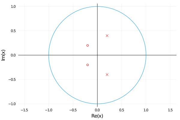
These plots show where a filter's Transfer Function explodes to infinity (poles, x on plot) or goes to zero (zeros, circle on plot):
Unfortunately, I was having a hard time connecting these visualizations with the way a filter "sounds". There's a number of interactive "filter explorer" tools available, but, for the sake of learning/understanding, I decided to build my own.
My filter explorer more or less does one thing: convert a polynomial from one form to another. This took me more time than it should have; I already knew most of what I needed to know, but had some trouble putting the tools together. Fortunately, it was fun to figure this out, so here's the whole story, including the missteps.
Symbolic Pole-Zero expansion
A Pole-Zero plot implies a transfer function in this form (\(q_i\) are zeros and all \(p_i\) are poles):
\[ H(z) = \frac{ (1-q_1 z^{-1})(1-q_2 z^{-1}) \ldots (1-q_M z^{-M}) }{ (1-p_1 z^{-1})(1-p_2 z^{-2}) \ldots (1-q_N z^{-N}) } \]
To actually run the filter (using the WebAudio IIRFilter class, for example), we need to get the function into this form:
\[ H(z) = \frac{ B(z) }{ A(z) } = \frac{ b_0 + b_1 z^{-1} + b_2 z^{-2} + \ldots + b_M z^{-M} }{ 1 + a_1 z^{-1} + a_2 z^{-2} + \ldots + z_N z^{-N} } \]
Basically, we need to go from \((1-q_1 z^{-1})(1-q_2 z^{-1}) \ldots\) to \(b_0 + b_1 z^{-1} + b_2 z^{-2} + \ldots\).
There are many polynomials with the same roots (\(gB(z)\) and \(B(z)\) have same roots), so we'll just pick the polynomial that is easiest to generate (let \(b_0 = 1\)). This algebra is pretty straightforward by hand or with a computer algebra system.
Closed Form (Wild Goose Chase)
I correctly didn't want to import an entire Computer Algebra System into my app to do this algebra. I incorrectly assumed that doing the multiplication without a computer algebra system would be tricky. In retrospect, I already knew how to easily multiply polynomials (see next section), but my brain-map didn't connect these topics so I went on a wild goose chase.
I decided to see if there was a closed form expression for the \(b_i\) coefficient written in terms of the roots \(q_j\).
Consider the following:
\[ \begin{aligned} \prod\nolimits_{i=1}^{2} (1-q_i z_{-1}) &= 1 \\ &- (q_1 + q_2) z^{-1} \\ &+ (q_1 q_2) z^{-2} \\ \prod\nolimits_{i=1}^{3} (1-q_i z_{-1}) &= 1 \\ &- (q_1 + q_2 + q_3) z^{-1} \\ &+ (q_1 q_2 + q_1 q_3 + q_2 q_3) z^{-2} \\ &- (q_1 q_2 q_3) z^{-3} \\ \prod\nolimits_{i=1}^{4} (1-q_i z_{-1}) &= 1 \\ &- (q_1 + q_2 + q_3 + q_4) z^{-1} \\ &+ (q_1 q_2 + q_1 q_3 + q_1 q_4 + q_2 q_3 + q_2 q_4 + q_3 q_4) z^{-2} \\ &- (q_1 q_2 q_3 + q_1 q_2 q_4 + q_1 q_3 q_4 + q_2 q_3 q_4) z^{-3} \\ &+ (q_1 q_2 q_3 q_4) z^{-4} \end{aligned} \]
It looks like there might be straightforward closed form for any of these coefficients (pardon the awkward notation):
\[ \begin{align} b_0 &= 1 \\ b_i &= (-1)^i \sum_{ Q \in \text{combs}(i) } \bigg[ \prod_{ j \in Q } q_j \bigg] \end{align} \]
Where \(\text{combs}(i): \mathbb{Z} \mapsto \mathbb{Z}^i\) is the set of all length-\(i\) combinations of coefficients.
Here's a possibly even harder to understand version in Julia/SymPy:
z = symbols("z")
function build_expr(n_roots)
    qs = symbols("q1:$(n_roots+1)") # generates q1,q2,...

    poly = 1
    for i in 1:n_roots
        prods = [reduce(*, c) for c in combinations(qs, i)]
        poly += ((-1)^i * reduce(+, prods))/z^i
    end
    return poly
end
Again, using SymPy, it's trivial to test if the code works for a given number of roots:
function test_expr(n_roots)
    mine = build_expr(n)

    # first generate the actual solution
    qs = symbols("q1:$(n_roots+1)") # generates q1,q2,...
    actual = reduce(*, [(1-qs[i]/z) for i in 1:n])

    # if these exprs cancel out, then the exprs are equivalent
    return (mine - actual).expand() == 0
end

test_expr(1) # true
test_expr(2) # true
test_expr(3) # true
test_expr(4) # true
test_expr(5) # true... must be correct!
This result is kind of cool, but not particularly easy to compute. I'm also not quite sure how to prove correctness. Filter-function-form conversion seems like it should be pretty common, so I figured if I google around using terms like "polynomial coefficients" and "combinations," I'd find some references to this method right away.
Wrong!
A few things I did find are:
- Pascal's Triangle (similar structure, solving a different problem).
- Polynomial interpolation techniques (fitting a polynomial through the zeros).
- A stack overflow post referencing Vieta's formulas (has the same structure)
- Characteristic Polynomial of a Matrix. Slightly different problem, but has a similar form.
- Elementary Symmetric Polynomials. Wikipedia page that ties all of the above together
Alright, I'm reasonably convinced that this method is correct, I just don't quite have the abstract math tools to reason whatever mathematical object I'm manipulating.
What I couldn't find was any references to using this sum-of-products-of-combinations approach to find filter coefficients. If I'm not finding references to this method it must not be a common technique.
I decided to go back to the JOS book and look for inspiration again. The very lucky/very ADD story:
- Read the book (Chapter on Partial Fraction Expansion)
- Realize that the matlab
residuezfunction is doing "filter function form" manipulation, kind of. - Go to matlab docs; Click through all of the additional "see more" functions referenced in the matlab help for
residuez. - Find the obviously-named
tf2zpkfunction, which does the opposite of what I want. - If
tf2zpkexists, maybezpk2tfalso exists? Google that. - It does. In SciPy. Read SciPy docs for
zpk2tf. The function: "Return[s] polynomial transfer function representation from zeros and poles"
Ah ha!
zpk2tf is exactly what I've been looking for.
Next question, what does zpk2tf do?
The Correct Way
I grab the scipy source and start reading.
The function zpk2tf essentially just calls a numpy function poly to compute the coefficients of the polynomials \(A(z)\) and \(B(z)\) from their respective roots.
Aside: the docs for `np.poly` reference characteristic polynomials, so there some relationship here!
np.poly is very simple: it just does some convolutions.
Polynomial multiplication is just convolution of the polynomial coefficients (something I already knew, but didn't connect to this problem).
For example, the polynomial \(1 + 2x + 3x^2\) can be represented as the list [1, 2, 3].
Then, to multiply \((1+2x+3x^2)(1-2x)\), we'd just need to conv( [1,2,3], [1,-2] ).
This produces the expected result [1, 0, -1, -6], or \(1 - x^2 - 6x^3\)
So, in psuedo-python, the entire roots-to-coefficients transformation boils down to:
poly = [1.0]                 # start with the polynomal "1"
for root in roots:
    term = [1.0, -root]      # the term 1 - (q_i)x
    poly = conv(poly, term)  # multiply in new term for this root
In other words, we can just repeatedly multiply each \((1-q_i z^{-1})\) term into a final polynomial using a speedy convolution. This is obviously much simpler than the nonsense above, so this is the method that my filter explorer uses.