A project I've been working on recently requires that I set a group of pins (4 of them) on a Teensy 4.1 to certain values at roughly the same time. For simplicity, I'm using the Arduino libraries for this project (but writing C++). We can fortunately easily look under the covers with the Teensy's Arduino implementation. In this post I'm going to walk through a few bad ways this can be done, and the correct way (for Teensy 4.1).
The simplest possible way to set multiple pins is to just set them one at a time.
For example, we could write:
int main( void ) { // configure a few pins as output pins pinMode( 23, OUTPUT ); pinMode( 22, OUTPUT ); pinMode( 21, OUTPUT ); pinMode( 20, OUTPUT ); int state = 0; while( 1 ) { asm volatile( "@ --- writes happen here" ); // helpful for navigating generated asm digitalWriteFast( 23, state ); digitalWriteFast( 22, state ); digitalWriteFast( 21, state ); digitalWriteFast( 20, state ); asm volatile( "@ --- done with writes" ); // toggle state and wait for a bit state = !state; delayMicroseconds( 10 ); } }
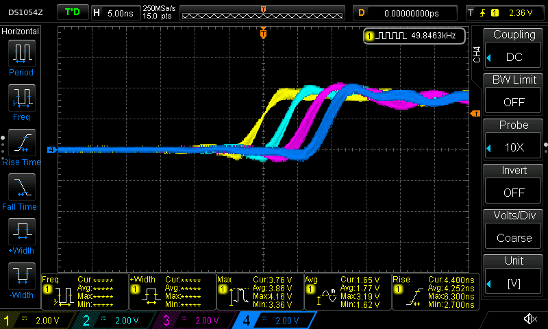
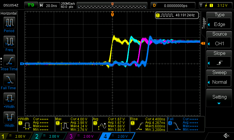
Compiling and running this code against a teensy and some LEDs, we can see (if we bump up the delay) that the lights flash on and off at about the same time. Let's try measuring the behavior with a slightly better tool than our eyes. I connected each pin to an oscilloscope. Channel 1 is pin 23, channel 2 is pin 22, and so on.
Let's take a look at both the:
state
was 0, is now 1. The pin output moves from 0V to 3.3Vstate
was 1, is now 0. The pin output moves from 3.3V to 0V.Rising edge:
Falling edge:
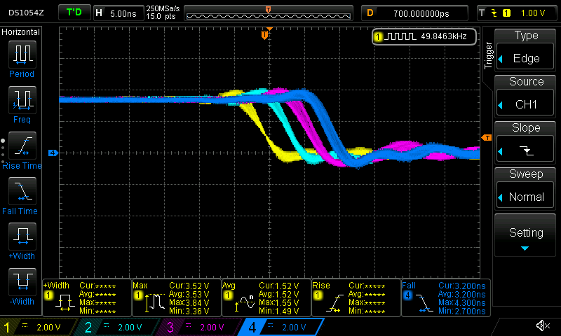
The scope conveniently measured a roughly 4ish nanosecond rise time and a 3ish ns fall time for each individual pin outputs. This is pretty fast (I think) for each individual pin, but for this project I want to set all of the pins at the same time.
These pin outputs are clearly not changing at the same time. Eyeballing, pin 23 reaches it's steady state output value roughly 4-5ish nanoseconds before pin 22.
Of course, this should not be surprising given that the code is setting the pin values one at a time.
Let's dig in.
This code compiles to something much more complicated that the simple "set pin x to value v" function calls would indicate. The Teensy 4.1 doesn't actually have any facility with which it can set a single output pin!
Instead, the output pins are mapped to GPIO port. Each port controls some number of pins, and, any assignment to a port will change the state of all the pins controlled by that port.
These ports are "mapped" into memory at well-documented address. To write to a port from a program running on the Teensy, the program just needs to write a value to a well-known address in memory (also called "registers"). When the memory system for the microcontroller observes a store to these magic addresses, it will do the electrical magic required to change the voltage on the appropriate pins.
For each port, there are two registers that we care about (and one that we could use, but aren't):
When writing to each of these registers, we supply a bitmask of the pins to modify.
For example, we could write a mask like 1010
to some "set" register to turn on every other pin, then write 1010
to a "clear" register to turn them all off again.
Rephrasing the code above in these terms, we actually are doing something like:
int state = 0; while( 1 ) { if( state ) { assign_to_set_register( 0b1000 ); // turn on Pin 1 assign_to_set_register( 0b0100 ); // turn on Pin 2 (Pin 1 stays on) assign_to_set_register( 0b0010 ); // turn on Pin 3 (Pin 1 and 2 stay on) assign_to_set_register( 0b0001 ); // turn on Pin 4 (Pin 1, 2, and 3 stay on) } else { assign_to_clear_register( 0b1000 ); // turn off Pin 1 (Pin 2, 3, 4 stay on) assign_to_clear_register( 0b0100 ); // turn off Pin 2 (Pin 3, and 4 stay on) assign_to_clear_register( 0b0010 ); // turn off Pin 3 (Pin 4 stays on) assign_to_clear_register( 0b0001 ); // turn off Pin 4 } }
Expressed this way, it looks really silly! We should clearly just turn on every pin on in the first assignment (we'll get there, be patient).
Inspecting the generated assembly code (which is actually how I figured out what is going on), we can see this behavior:
; compute the bitmask values into r9, r8, ip, lr ; ; .... some other code .... ; ; --- turn on using the SET registers str r9, [r4, #132] @ tmp149, MEM[(struct IMXRT_GPIO_t *)1107296256B].DR_SET str r8, [r4, #132] @ tmp150, MEM[(struct IMXRT_GPIO_t *)1107296256B].DR_SET str ip, [r4, #132] @ tmp151, MEM[(struct IMXRT_GPIO_t *)1107296256B].DR_SET str lr, [r4, #132] @ tmp152, MEM[(struct IMXRT_GPIO_t *)1107296256B].DR_SET ; ; .... some other code .... ; ; --- turn off using the CLEAR registers str r9, [r4, #136] @ tmp149, MEM[(struct IMXRT_GPIO_t *)1107296256B].DR_CLEAR str r8, [r4, #136] @ tmp150, MEM[(struct IMXRT_GPIO_t *)1107296256B].DR_CLEAR str ip, [r4, #136] @ tmp151, MEM[(struct IMXRT_GPIO_t *)1107296256B].DR_CLEAR str lr, [r4, #136] @ tmp152, MEM[(struct IMXRT_GPIO_t *)1107296256B].DR_CLEAR
In this code above, r4
contains a base address for the list of registers.
The offset [r4, #132]
contains the SET register for the pins we care about and [r4, #136]
is the CLEAR register.
As demonstrated by the scope, we see a small (but predictable) amount of latency on each of these sets because we're running 4 store instructions in quick succession. But, of course, we can do much better than this by getting away from the arduino apis.
It's easy to implement the appropriate GPIO port code by grabbing bits and pieces from the teensy arduino headers.
int main( void ) { // use ardino functions for configuration uint8_t pins[] = { 23, 22, 21, 20 }; for( size_t i = 0; i < ARRAY_SIZE( pins ); ++i ) { pinMode( pins[i], OUTPUT ); } // bit pattern to set/clear bits // use the helpful bit patterns defined by core_pins.h as part of teensy support code uint32_t pattern = CORE_PIN23_BITMASK | CORE_PIN22_BITMASK | CORE_PIN21_BITMASK | CORE_PIN20_BITMASK; int state = 0; while( 1 ) { asm volatile( "@ --- writes happen here" ); // helpful for navigating generated asm if( state ) { GPIO6_DR_SET = pattern; // turn pins on with SET register } else { GPIO6_DR_CLEAR = pattern; // turn pins off with CLEAR register } asm volatile( "@ --- done with writes" ); state = !state; delayMicroseconds( 10 ); } }
The generated assembly does exactly what we're looking for:
; -- set str r7, [lr, #132] @ tmp175, MEM[(struct IMXRT_GPIO_t *)1107296256B].DR_SET ; -- clear str r7, [lr, #136] @ tmp175, MEM[(struct IMXRT_GPIO_t *)1107296256B].DR_CLEAR
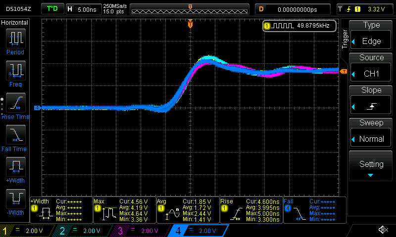
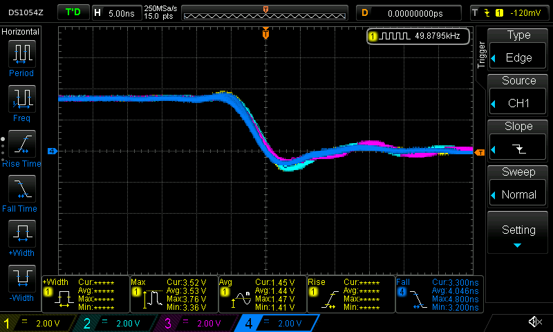
And, the scope shows a much nicer shape for both the rising edge and falling edge:
The Arduino APIs are fantastically useful for getting started quickly, but dropping to lower level APIs can be important. Fortunately, the Teensy makes it fantastically easy to dig around and use the chip when needed, and, the headers are even documented with where to look in the official manual! Awesome product.
I'm always looking for tools that have both a quick-and-easy beginner API, but don't necessarily sacrifice on depth for advanced use. So far the Teensy is filling that role well.
Suppose we replace the code with something a bit more flexible (and that was recommended in the arduino forums).
#define ARRAY_SIZE( arr ) (sizeof(arr)/sizeof(*arr)) extern "C" int main( void ) { uint8_t pins[] = { 23, 22, 21, 20 }; for( size_t i = 0; i < ARRAY_SIZE( pins ); ++i ) { pinMode( pins[i], OUTPUT ); } int state = 0; while( 1 ){ asm volatile( "@ --- writes happen here" ); // helpful for navigating generated asm for( size_t i = 0; i < ARRAY_SIZE( pins ); ++i ) { digitalWriteFast( pins[i], state ); } asm volatile( "@ --- done with writes" ); state = !state; delayMicroseconds( 10 ); } }
Something bad clearly happens when we run this code:
First, we notice that the time delta between writes has increased dramatically. Second, we notice that the pin 23 and ping 22 write are further apart in time than the pin 22 and pin 21 write.
What happened?
The inner assignment loop this time compiled into:
@ --- writes happen here add r3, sp, #4 @ tmp202,, .L5: ldrb r2, [r3], #1 @ zero_extendqisi2 @ D.14694, MEM[base: _138, offset: 0B] lsls r2, r2, #4 @ tmp168, D.14694, adds r0, r6, r2 @ tmp169, tmp193, tmp168 ldr r2, [r6, r2] @ D.14697, ldr r0, [r0, #12] @ D.14698, cbz r5, .L3 @ state, str r0, [r2, #132] @ D.14698, MEM[(volatile uint32_t *)_22 + 132B] .L4: cmp r3, r4 @ ivtmp.15, D.14699 bne .L5 @, @ --- done with writes
Inspecting the source for digitalWriteFast
we can see that we've taken the non-compile-time-constant code path:
static inline void digitalWriteFast(uint8_t pin, uint8_t val) { if (__builtin_constant_p(pin)) { if (val) { if (pin == 0) { CORE_PIN0_PORTSET = CORE_PIN0_BITMASK; } else if (pin == 1) { // ..... } // ..... } else { if (pin == 0) { CORE_PIN0_PORTCLEAR = CORE_PIN0_BITMASK; } else if (pin == 1) { // ..... } // ..... } } else { // not a compile time constant if(val) *portSetRegister(pin) = digitalPinToBitMask(pin); else *portClearRegister(pin) = digitalPinToBitMask(pin); }
I'm guessing that the variability has something to do with additional memory access (lookups to figure out pin maps to what register). This probably could have compiled down to use all compile time constants, but this massive change in behavior for roughly the same code is reasonably spooky.
Many DSP resources use "pole-zero" plots to compactly represent audio filters.
These plots show where a filter's Transfer Function explodes to infinity (poles, x
on plot) or goes to zero (zeros, circle on plot):
Unfortunately, I was having a hard time connecting these visualizations with the way a filter "sounds". There's a number of interactive "filter explorer" tools available, but, for the sake of learning/understanding, I decided to build my own.
My filter explorer more or less does one thing: convert a polynomial from one form to another. This took me more time than it should have; I already knew most of what I needed to know, but had some trouble putting the tools together. Fortunately, it was fun to figure this out, so here's the whole story, including the missteps.
A Pole-Zero plot implies a transfer function in this form (\(q_i\) are zeros and all \(p_i\) are poles):
\[ H(z) = \frac{ (1-q_1 z^{-1})(1-q_2 z^{-1}) \ldots (1-q_M z^{-M}) }{ (1-p_1 z^{-1})(1-p_2 z^{-2}) \ldots (1-q_N z^{-N}) } \]
To actually run the filter (using the WebAudio IIRFilter
class, for example), we need to get the function into this form:
\[ H(z) = \frac{ B(z) }{ A(z) } = \frac{ b_0 + b_1 z^{-1} + b_2 z^{-2} + \ldots + b_M z^{-M} }{ 1 + a_1 z^{-1} + a_2 z^{-2} + \ldots + z_N z^{-N} } \]
Basically, we need to go from \((1-q_1 z^{-1})(1-q_2 z^{-1}) \ldots\) to \(b_0 + b_1 z^{-1} + b_2 z^{-2} + \ldots\).
There are many polynomials with the same roots (\(gB(z)\) and \(B(z)\) have same roots), so we'll just pick the polynomial that is easiest to generate (let \(b_0 = 1\)). This algebra is pretty straightforward by hand or with a computer algebra system.
I correctly didn't want to import an entire Computer Algebra System into my app to do this algebra. I incorrectly assumed that doing the multiplication without a computer algebra system would be tricky. In retrospect, I already knew how to easily multiply polynomials (see next section), but my brain-map didn't connect these topics so I went on a wild goose chase.
I decided to see if there was a closed form expression for the \(b_i\) coefficient written in terms of the roots \(q_j\).
Consider the following:
\[ \begin{aligned} \prod\nolimits_{i=1}^{2} (1-q_i z_{-1}) &= 1 \\ &- (q_1 + q_2) z^{-1} \\ &+ (q_1 q_2) z^{-2} \\ \prod\nolimits_{i=1}^{3} (1-q_i z_{-1}) &= 1 \\ &- (q_1 + q_2 + q_3) z^{-1} \\ &+ (q_1 q_2 + q_1 q_3 + q_2 q_3) z^{-2} \\ &- (q_1 q_2 q_3) z^{-3} \\ \prod\nolimits_{i=1}^{4} (1-q_i z_{-1}) &= 1 \\ &- (q_1 + q_2 + q_3 + q_4) z^{-1} \\ &+ (q_1 q_2 + q_1 q_3 + q_1 q_4 + q_2 q_3 + q_2 q_4 + q_3 q_4) z^{-2} \\ &- (q_1 q_2 q_3 + q_1 q_2 q_4 + q_1 q_3 q_4 + q_2 q_3 q_4) z^{-3} \\ &+ (q_1 q_2 q_3 q_4) z^{-4} \end{aligned} \]
It looks like there might be straightforward closed form for any of these coefficients (pardon the awkward notation):
\[ \begin{align} b_0 &= 1 \\ b_i &= (-1)^i \sum_{ Q \in \text{combs}(i) } \bigg[ \prod_{ j \in Q } q_j \bigg] \end{align} \]
Where \(\text{combs}(i): \mathbb{Z} \mapsto \mathbb{Z}^i\) is the set of all length-\(i\) combinations of coefficients.
Here's a possibly even harder to understand version in Julia/SymPy:
z = symbols("z") function build_expr(n_roots) qs = symbols("q1:$(n_roots+1)") # generates q1,q2,... poly = 1 for i in 1:n_roots prods = [reduce(*, c) for c in combinations(qs, i)] poly += ((-1)^i * reduce(+, prods))/z^i end return poly end
Again, using SymPy, it's trivial to test if the code works for a given number of roots:
function test_expr(n_roots) mine = build_expr(n) # first generate the actual solution qs = symbols("q1:$(n_roots+1)") # generates q1,q2,... actual = reduce(*, [(1-qs[i]/z) for i in 1:n]) # if these exprs cancel out, then the exprs are equivalent return (mine - actual).expand() == 0 end test_expr(1) # true test_expr(2) # true test_expr(3) # true test_expr(4) # true test_expr(5) # true... must be correct!
This result is kind of cool, but not particularly easy to compute. I'm also not quite sure how to prove correctness. Filter-function-form conversion seems like it should be pretty common, so I figured if I google around using terms like "polynomial coefficients" and "combinations," I'd find some references to this method right away.
Wrong!
A few things I did find are:
Alright, I'm reasonably convinced that this method is correct, I just don't quite have the abstract math tools to reason whatever mathematical object I'm manipulating.
What I couldn't find was any references to using this sum-of-products-of-combinations approach to find filter coefficients. If I'm not finding references to this method it must not be a common technique.
I decided to go back to the JOS book and look for inspiration again. The very lucky/very ADD story:
residuez
function is doing "filter function form" manipulation, kind of.residuez
.tf2zpk
function, which does the opposite of what I want.tf2zpk
exists, maybe zpk2tf
also exists? Google that.zpk2tf
. The function: "Return[s] polynomial transfer function representation from zeros and poles"
Ah ha!
zpk2tf
is exactly what I've been looking for.
Next question, what does zpk2tf
do?
I grab the scipy source and start reading.
The function zpk2tf
essentially just calls a numpy function poly
to compute the coefficients of the polynomials \(A(z)\) and \(B(z)\) from their respective roots.
Aside: the docs for `np.poly` reference characteristic polynomials, so there some relationship here!
np.poly
is very simple: it just does some convolutions.
Polynomial multiplication is just convolution of the polynomial coefficients (something I already knew, but didn't connect to this problem).
For example, the polynomial \(1 + 2x + 3x^2\) can be represented as the list [1, 2, 3]
.
Then, to multiply \((1+2x+3x^2)(1-2x)\), we'd just need to conv( [1,2,3], [1,-2] )
.
This produces the expected result [1, 0, -1, -6]
, or \(1 - x^2 - 6x^3\)
So, in psuedo-python, the entire roots-to-coefficients transformation boils down to:
poly = [1.0] # start with the polynomal "1" for root in roots: term = [1.0, -root] # the term 1 - (q_i)x poly = conv(poly, term) # multiply in new term for this root
In other words, we can just repeatedly multiply each \((1-q_i z^{-1})\) term into a final polynomial using a speedy convolution. This is obviously much simpler than the nonsense above, so this is the method that my filter explorer uses.
I've recently been toying around with different headset setups for zoom/casual online gaming (with voice) with friends.
As part of this experiment, I decided to try out a pair of true wireless bluetooth earbuds, but was astonished by how terrible the audio latency seemed to be.
In a (failed) attempt to measure the latency, I wrote these two little web "apps":
Note: not sure if either of them work on iOS. Something seems to be broken, but debugging on iOS apparently requires owning a macbook.
With (2), I was hoping that my response time variance would be low enough to effectively measure the bluetooth latency by comparing my audio and visual response times. This doesn't seem to be the case, my response times are all over the place.
Likely I'll keep toying with how to measure this, maybe some fancy apparatus that records the audio my headphones hear?
]]>I've built a micro-benchmark which sends data between CPU 2 cpu cores. On my single AMD 3800X desktop CPU, I have crafted a microbenchmark which has different performance characteristics depending on pair of cores I select for testing.
Results like this should not be surprising on a multi-socket system, but this system has only a single processor. I believe this micro-benchmark is highlighting some of the features of the novel architecture on the new AMD chips.
Before diving in to Zen, I'd like to talk briefly CPU memory-caching systems.
Modern CPUs contain a variety of fast memory which cache accesses to the larger more expensive RAM. Usually we call the fastest, smallest cache L1, the next fastest L2, and the largest, but slowest cache L3. These caches communicate with each other to move data around (see MESI protocol).
Assume for simplification that the L3 cache knows how to get data from main memory or from the L1 and L2 caches. Also assume that the L3 cache is the only part of the memory system which is able to talk main memory.
If Core 0 wants to read from memory, it will ask the local L1 cache to perform the read. If the data is in the L1 cache, the cache sends the data to the CPU registers. If the data is not in the L1 cache, the cache asks L2. Finally, the L2 cache asks L3 and the L3 cache goes and fetches the data.
Next, assume that all data is written into the L1 cache then propagated out to other caches or main memory as needed. When the L1 cache is out of space, it will evict the data into the L2 cache. When the L2 cache is out of space, it will evict the data into the L3 cache. Finally, if L3 runs out of space, it will evict the data back to main memory.
Generally, each CPU has it's own L1 and L2 cache, but the L3 cache is shared by all of the cores. Something like this:
/-----------------------------------\ | | | L3 cache (shared by all cores) | | | +--------+--------+--------+--------+ | | | | | | L{1,2} | L{1,2} | L{1,2} | L{1,2} | | | | | | +--------+--------+--------+--------+ | | | | | | Core | Core | Core | Core | | | | | | \--------+--------+--------+--------/
This style of L1/L2/L3 cache has been common in CPU designs for many years.
To talk about AMD's Zen architecture, there's a few terms we need to define:
Each Ryzen processor has one IO controller and some number of CCD dies. This CCD/CCX/IO controller strategy allows AMD to mass produce CCD chips, performance/correctness test the cores (this is called "binning"), then build a wide variety of different processor configurations.
The particular Ryzen 3800X I own has a single IO controller and a single CCD. The CCD contains two CCXs. Each CCX in my particular CPU has all 4 physical cores enabled. Each of those physical cores is capable of running two threads (see Simultaneous Multithreading (SMT)).
Here's how this looks in hwloc's lstopo
output:
Interpreting the output, we can see that:
This likely means that cores in the same CCX can communicate with each other by reading and writing to their shared L3 cache. If cores from different CCXs need to communicate, they will have to use the infinity interconnect.
To verify my hypothesis, lets start with a classic pingpong roundtrip latency test.
This test runs two threads. The first thread flips a value in memory to some value "Ping", then waits to see another value "Pong." The second thread waits to see "Ping", then flips the value to "Pong."
The first thread starts timing right before sending "Ping", and stops timing once it sees "Pong."
I've plotted the mean core-to-core pingpong round-trip time for all pairs of cores (including the SMT cores). Latency for A->B and B->A were both tested (for no particular reason).
That is:
for core1 in cores: for core2 in cores: if core1 == core2: continue # skip self, both threads spin results[ (core1, core2) ] = mean_of_many_tests( core1, core2 )
This plot is a heatmap of core->core pingpong roundtrip time, in nanoseconds:
As we can see, there's a clear difference in round-trip latency between pairs of cores in the same CCX and pairs of cores in a different CCX. For example, core 0->core 3 round-trip latency is pinkish, but core 0->core 4 latency is dark blueish. The actual values I got around ~96ns for 0->3 and ~196ns for 0->4.
I do not have a good explanation for the upper and lower diagonal lines (at around 48ish ns), but, we can clearly see that pairs of cores for which latency was low share a common L3 cache (they are in the same CCX).
For full details about this benchmark, please see the source and my results here.
So, we know that there is a difference in latencies, but, does this really matter? Few applications actually have any reason to bounce a single value back and forth between cores.
When discussing latency, programmers who are more bandwidth focused will often (rightly) say something like "the latency doesn't matter, I only care about bandwidth." Most programmers are more focused on bandwidth than latency, because generally we care a lot more about throughput than latency.
Let's start by proving that, when moving around large chunks of data, none of this matters.
I've created a small tester which:
The region of memory that I am copying is 4 gigs large.
This is much larger than any of the local caches.
We should be able fire off a memcpy
then sit back while the hardware prefetchers and cache hierarchy work their latency-hiding magic.
Here's the plot:
As we can see, we're pretty much getting a ~14.5-15 GiB/s copy rate regardless of the cores selected. This is good news. The new AMD core layout makes no difference when copying around 4 gig chunks of data.
For full details about this benchmark, please see the source and my results here.
We are often able to amortize high latency operations over large transfers or by work on something else to hide the costs of high latency. However, as data sizes shrink, it becomes harder and harder to hide latency.
Recently, it seems like (anecdotally) there has been a trend of using queues to move data/send commands in throughput-oriented applications.
When messages sent over these queues are small, we might be able to observe Ryzen's latency characteristics as a drop in throughput.
I've built a simple microbenchmark to test this. The benchmark runs a writer thread and some number of reader threads. The threads share a region of memory that contains a bunch of "chunks". The array of chunks looks sort of a like a single producer, single consumer queue:
typedef struct { uint64_t ready; char padding[ CACHE_LINE_SIZE - sizeof( uint64_t ) ]; char data[ N_DATA_LINES*CACHE_LINE_SIZE ]; } chunk_t;
The ready
marker acts like a boolean.
The ready
marker always sits at the start of a cache line.
The size data
of the data region is always some multiple of the cache line size.
Padding is introduced to ensure that the data region and the ready
marker are not ever in the same cache line.
In pseudocode, the writer looks something like this:
for( size_t i = 0; i < N_CHUNKS; ++i ) { populate_chunk_data( &chunks[i] ); // signal that the reader should read the data atomic_store( &chunks[i].ready, true ); }
The reader looks something like this:
for( size_t i = 0; i < N_CHUNKS; ++i ) { // Wait for the chunk to be ready while( !atomic_load( &chunks[i].ready ) ) { } read_and_discard_data( &chunks[i] ); }
In theory, chunk transfer will occur one at a time when the reader and the writer are running at more or less the same speed. If the reader falls behind the writer, the writer should be able to plow ahead with its writes and the reader should be able to continue reading until it catches up or finishes.
In the benchmark, I've placed the array of chunks into a 2 megabyte huge page. I created a region containing 8192 chunks, and each chunk's data segment contains 8 cache lines (512 bytes) of data. The number of chunks doesn't seem to affect the benchmark much, but the size of the data segment does. I've kept the size low to highlight the effects I'm looking for, but, these effects seem to still be present for data sizes up to a few KiB.
Using the same style of plots that we've already see, let's first look at bandwidth reported by the writer. This plot shows the write rate when Y-axis core is sending data to X-axis core (rate is in GiB/s, I've again included the SMT cores):
There's some patterns in this plot that I have not been able to explain, but, there doesn't seem to be any significant variation in write rate when the reader core is on a different CCX. I'm reasonably confident claiming that the writer is unaffected by choice of core.
Here's the rates that the reader reported:
From the reader's perspective, the differences are stark. When the reader and writer share an L3 cache (are in the same CCX), we consistently see a read rate around 13-14 GiB/s. When the reader and writer do not share the L3 cache (are in different CCX), the read rates are consistently lower, around 10-11 GiB/s.
This is a significant enough difference to warrant careful attention when building high performance software.
For full details about this benchmark, please see the source and my results here.
This sort of behavior will not come as a surprised for programmers used to programming for multi-socket (multiple physical CPU) server systems (see NUMA). However, for those writing parallel applications, I feel like this effect is still notable and warrants slightly different considerations than traditional NUMA.
In a traditional multi-socket/multiple-physical CPU system, RAM is physically connected to only one of the many CPUS. If core0 of cpu0 needs to access memory physically attached to cpu1, it will pay a latency penalty to access this memory (this is NUMA - Non-Uniform Memory Access). However, we've also generally assumed that core0 can access any part of memory attached to cpu0 with the same latency. Therefore, applications built for NUMA architectures often focused on getting their data into the memory CPU attached to a CPU, then using the cores on that CPU to process the data.
For platforms like AMD's (and recent Intel, see Intel Mesh) we have to now make NUMA-style considerations any time we are operating over a piece of data on multiple cores, not just when dealing with multiple sockets.
Consider the specs for the EPYC 7542:
On the 7542, we have to divide this 128 MiB of L3 cache up into CCX cache slices. Assuming each CCX has 4 cores (which I think is correct), we'd have 32/4=8 CCXs on this CPU. Therefore, each CCX (4 cores) only has 16 MiB of "close L3 cache memory," accessing the rest of the cache will incur a small amount of extra latency.
For comparison, a 2016 Intel Broadwell Xeon could be configured with 22 cores and 55 MiB of L3 cache. This means that the AMD has a core/fast-shared-l3 ratio of 0.25 MiB/core and the Broadwell has a core/fast-shared-l3 ratio of 2.5 MiB/core. Building high performance code with 2.5 MiB of super fast shared memory per core is a slightly different game than building high performance applications with only 0.25 MiB of super fast shared memory per core.
I suspect that "networked" cpu architectures will become the new normal in the next few years. These new platforms are going probably going to be increasingly more and more sensitive to data access and data movement than the systems of the past.
For the last 192 days (according to uptime on one my routers), I've been setting up a small homelab. Homelabs are kind of cool, and, the setup has been interesting. I'll be writing a few posts explaining the steps I took.
Now that I have a VPN, a server, a "desktop computer" connected to the server over a fast network, and fast storage, I should do something useful.
These tools are useful for general system monitoring.
Also, grafana plots are really pretty:
I'm also a fan of using these tools to report your own metrics from your own small applications. You can very easily write stats to output files then jam them through telegraf to collect them and produce plots. See https://github.com/influxdata/telegraf/blob/master/docs/DATA_FORMATS_INPUT.md.
healthchecks.io is an altering service that sends alerts through email, slack, etc when it hasn't received a ping recently enough. You can run the open-source software yourself, or use a hosted version.
To set it up, you register a number of "checks" and assign each check a schedule:
Sending updates is also trivial; I just use use curl
to send "stating", "failed," and "succeeded" messages from a shell script:
#!/bin/bash set -o pipefail # don't set -e because we want failure to make it all the way to the end, not # sure that's actually happening here # retrying curl is questionable if [ "$#" -lt 2 ]; then echo "Usage: URL cmd..." exit 1 fi url=$1 echo "Sending start message" curl --silent -fsS --retry 3 -X GET ${url}/start echo # run the rest of the arguments as a command ${@:2} rc=$? if [ ${rc} -eq 0 ]; then echo "Success" curl --silent -fsS --retry 3 -X GET ${url} # done! echo else echo "Command ${@:2} failed" echo "Sending fail message" curl --silent -fsS --retry 3 -X GET ${url}/fail echo fi exit ${rc}
Sending start/{success,fail} messages is helpful because:
Backups are tricky.
My requirements:
For many years I've used and recommended CrashPlan. I still would recommend CrashPlan; their service satisfies almost all of the above requirements.
On a recent backup test though, I found their recovery to be somewhat slow. I decided to see what else is available.
After assessing many of the open-source options, I settled on duplicacy and Backblaze B2 for a first experiment. Duplicacy satisfies many of thes objectives:
So far, this experiment has gone well.
Each backup set I have configured backs up on a timer using systemd and pings healthchecks with its status.
A few of the snapshots from my laptop were corrupted I believe because I closed my laptop lid at a bad time, but, my duplicacy check
job (which also reports to healthchecks), quickly noticed the issue and I was alerted.
Setting this up obviously takes more work than just downloading CrashPlan, but, so far I've been pretty happy with how this experiement has gone so I will be continuing it for now.
Nothing.
I've wanted to alert on a few things from log files, so I've just thrown a grep BAD_THING log_file
into a script, checked the return code, and alerted to healthchecks when the bad thing happened.
I don't need log searching/aggregation features for 3 computers.
The personal software development projects I work on can also take advantage of this server/vpn setup. I'm able to ssh into both of my home machines from anywhere (because of the VPN), so I always have access to the larger CPUs available there (very handy when compiling rust/c++ code).
I'm also using the server for:
I have a small archive of:
Saving these files on a backed-up, redundant storage system is working out well. Also, since I can NFS mount this drive over my VPN, I can get at the files anywhere that a computer is available. There's not a ton here, and there's not a ton that I want to keep readily accessible, so this is more of a dumping ground for things that I want to keep but don't otherwise need at my fingertips.
I currently do all of my music projects from an actual computer, so I'm storing all of the samples I've collected and recordings I've made on the NAS. Since I run linux everywhere, I can NFS mount this drive from anywhere in my apartment and access my samples.
As part of an experiment to try moving from GMail to literally anything else, I started trying to backup my emails and contacts. I'm using isync to download my emails, because it is extremely configurable. I have isync setup to:
This config looks something like (with right column annotations):
Channel mail Master :mail-remote: Slave :mail-local: Sync Pull All # Pull all changes from remote->local Patterns % !Trash # Don't sync the Trash folder Create Slave # If a directory is missing on the slave, create it Remove Slave # Remove directory from slave if it doens't exist on master CopyArrivalDate yes SyncState * Expunge Slave # Actually delete stuff on the slave if it gets deleted on master Channel mail-archive # mostly the same, but filters down to Trash only and never expunge Master :mail-remote: Slave :mail-local: Pattern Trash Sync Pull All Create Slave Remove slave CopyArrivalDate yes SyncState *
I'm running rss2email on the server to send RSS feeds to my email. Using a 32 core behemoth to run a python script daily is silly, but oh well.
rss2email works wonderfully and I highly recommend it. This came about for me because I wanted to read RSS feeds in emacs, but I also wanted to be able to mark stuff as read on my phone. My email is available on my phone, and I can make my email show up in emacs, so I'm trying this out.
WeeChat has a pretty nifty relay protocol that can be used to remotely access your WeeChat instance from a browser or mobile device. I've been running WeeChat on my machine instead of figuring out how to configure ZNC or some other bouncer. Im not super active on IRC, but I've been happy with this approach and these tools.
I have a large collection of RAW photos captured in a variety of vendor-specific RAW formats. Getting these onto storage I owned and controlled was the main reason I built my NAS server.
Up until recently, Adobe's cloud version of Lightroom (Lightroom CC) has worked really well for me.
However, on a recent trip a few deficiences started to stand out:
I tried to glue together pieces of open source software to get some important subset of the above features, but, this never totally worked.
The closest thing that currently exists is DigiKam with a Remote Database. DigiKam is a really great piece of software. Combine DigiKam with Darktable and rawtherapee and you'll have a truly wonderful desktop photo editing suite.
But, if you try to access your NFS photo collection over a crappy internet connection, even with the MySQL database, this isn't going to work out so well. Also, good luck doing anything with your phone.
I tried a bunch of crazy things to get this to work well from multiple machines and over poor internet connections, including keeping the entire DigiKam collection (and database) in git-annex.
For now, I'll be sticking with lightroom, but I'm keeping my eyes open for something better. I didn't trust any of the other solutions I came up with to be robust and reliable, and I didn't feel like I was gaining enough to give up the AI search, mobile editing, etc.
I don't mean for this to be an indictment of the open source stuff; the open source stuff is really good. The photo editing world just really hasn't caught onto the "cloud" thing yet. This space is also packed with proprietary software, proprietary file formats, and is sort of fundamentally unix-y. Adobe is the only company currently offering a cloud RAW editor with these nifty AI features. Everyone else that wants to use more than one machine generally has some crazy scheme involving Dropbox, partial syncing, and multiple databases (in flat files).
In a couple of months, I'll probably try this again. Maybe I'll even build my own editor/manager software that works perfectly and does everything.
I considered turning this into a media streaming box, but it's nearly impossible to legally obtain copies of most of the TV and movies I want to keep around. If I could easily get legal digital copies of the TV shows I want to watch, I'd be happy to pay, download, and manage the storage myself. This isn't the case, so I'm just going to keep unhappily renting all of the media I consume.
For music, I've been pretty happy keeping unique, hard to stream music sitting around in FLAC files in my junk archive, then uploading the albums to Google Play Music for streaming from my phone and office.
I'm currently using:
In theory, all of this could be done with orgmode, but I haven't been able to find a good way to sync org mode (with attachments) to mobile devices. More or less I've decided that I don't need to or want to actually write orgmode notes on a mobile device. I'm using todoist and email to send myself things I need to capture, then capturing them when I have a real computer. I can export everything as HTML for read only access on my phone, in a form factor that works well on a small screen (not yet automated or searchable).
I haven't figured out papers because I haven't tried to wrangle orgmode correctly to manage/tag/adjust metadata for them. Also, I regularly capture and sometimes read papers from my phone, so I need to find a proper workflow for managing these from my phone somehow.
Even if I could move all of this to orgmode, I'd still not be using the server for much of anything. In the best case, I'd have a handful of text files in a git repo (or nextcloud or something), and a pile of PDFs on the NAS. Again, none of this really requires a massive server.
Most of the things I use on a regular basis in my life outside of work aren't realistically replacable with self-hosted versions of things.
If I refuse to use facebook messenger (or facebook) to stay in touch with people, they simply will not stay in touch or invite me to events. Volunteer organizations I'm involved in use Google Docs to collaborate. All of my financial applications are closed off and nearly impossible to access with custom code. Lots of smart-junk needs to phone home to be fully functional.
I considered self-hosting email, but I'm not willing to deal with IP reputation issues and I'm not sure I want to have to keep my server running reliably enough to depend on it for email. I'm not going to self-host a password manager because I'll be royally screwed if my server goes down.
Since I like to jam the world into neat little dichotomies, here's some attempts explain why some things worked well for me and some things did not. I've come up with two ways to word this. I think they are equivalent:
I'm generally happy using developer tools, but generally unhappy when I interact with consumer products. I'm generally extremely comfortable convoluted keybindings or jamming together sed/grep/awk pipelines, but am often irritated when I get stuck in some tool that is "user friendly."
There's a few possible (hyperbolic) explanations:
grep
almost anything that lives in developer/sysadmin land. I can't grep
my gmail
.Reality is probably some combination of all of these.
Having an always-on machine, that I can get a virtual terminal on for adminstration has been convenient. Running my own DNS server with ad-blocking baked in has been fantastic. Having a rock-solid VPN server that I control, and that lets me ssh into my local machines from anywhere has been a game changer. Having a sweet server to occasionally run some tests or play with my 10 gig network is pretty great.
Using a High Powered Xeon Server to backup some files, sometimes send me some emails, and host a metrics database is absurd.
I'm disappointed that having my own server hasn't turned out to be more useful. Everything I use is a cloud service; everything I use to interact with other people is a cloud service. Many modern cloud services are simply better than their self hosted alternatives.
From a practial perspective, I'm most disappointed that I haven't managed to glue together or build something open source/self hosted to mange my photos.
For a more philosophical perspective, I'm really disappointed that I keep running up against walled gardens with opaque protocols. To be clear, I have no issue paying someone else to run services for me. I also don't really have any issue with services that use funky protocols, or even if the entire service is closed-source and super proprietary. I'm bothered that it is so difficult to move data between services and to easily hook things together to orchestrate some workflow I want.
In a perfect world, I'd be able to pay companies to host my email, do AI magic on my photos, provide storage for backups, etc. Then, ideally, I'd be able to glue this all together myself. I'd like to be able to move data between these services, bring my own storage, and build little custom tools to do cool tricks with the tools I have available.
In today's world, if I pay a company to host my email, I can't get push notifications on an Android phone, unless my email provider has built a custom app that uses google's servers to send messages to my phone (ironically the state of the world is very slightly better on apple devices).
In today's world, I can pay Adobe to host my photos, do magic AI stuff on them, and give me a nice editor, but I can barely get my photos out.
I can use Mendeley's free service to manage my PDFs, but I can't easily build a workflow that moves files between their cloud storage and my wifi-enabled eink reader (which can easily run custom code).
Maybe I just need to be patient and wait for all of these cloud products to become more mature. Maybe there's something in the fediverse (matrix and ActivityPub look promising) that solves some of these problems. Maybe I just need to move on and go do something more productive with my time..
For the last 172 days (according to uptime on one my routers), I've been setting up a small homelab. Homelabs are kind of cool, and, the setup has been interesting. I'll be writing a few posts explaining the steps I took.
In this homelab post, I'll be detailing how I converted the R720 I bought on eBay into a NAS server on my local network. This was an expensive project; I'm not sure it was worth the time or energy. I'll add more discussion on the usability of something like this in the 4th part of this series.
I recently had an old SSD fail. I had no idea it was going bad until I tried to open a handful of old photos and found that they were corrupt. Some of the smart counters for the drive apparently had ticked up, but I never had set up anything automated to monitor this, so it was missed. Of course, the files were all backed up, but this still isn't a great experience to have.
I wanted a safe place to store some important files. I wanted these files to be available on all of my devices. I didn't really want to use a cloud service for this, since I've been trying to scale back my cloud dependence and vendor lock-in problem (but maybe I should have).
For a local disk, I would certainly need some form of RAID array (and of course backups, but that's for a later post).
Currently in the root of the /nas
contains:
Right now, all of this is is only using about 500 gigs of space.
These files used to live on either 1) a spinning rust drive on my desktop or 2) my home directories on multiple machines (not really synced other occasional rsyncs of subsets of the data). This post will discuss setting up the ZFS and mounting it as a NAS.
Since I was only using about 500 gigs of space, I wasn't going to need some super high capacity system. I decided to instead try and build something that would be 1) lowish power (spinning rust is power hungry), 2) pretty "fast", 3) "fun".
Since this is all going into my only server, I'd also need some space for all of the other services I wanted to toy with, so I came up with this:
Data Category | Space | Speed | Redundancy |
---|---|---|---|
Personal Data | 2TB should last years | fast-ish | needs to be highly redundant |
server drive | 500GB more than enough | fast | doesn't need to be redundant |
OS drive | 500GB | fast | doesn't need to be redundant |
The server has 16 2.5 inch SAS/SATA drive bays connected to a "SAS backplane." The backplane is connected to a Dell-rebranded LSI hardware RAID controller card. The RAID controller card is connected to the CPU via 8 Gen 3 PCIe lanes (in a Dell-proprietary form factor slot).
The backplane on server hold 16 drives and has across 8 SAS ports. Each SAS port can do 6 Gbit/s, so we can do (6*8)/8 = 6 Gbytes/s on the RAID controller + backplane, in theory. This is well matched with the PCIe bandwidth, which is theoretically around 7.9 gigs a second.
The good thing about all of this is that the backplane/RAID controller were well integrated into Dell's remote management tools. The bad thing is of course that many of these parts are proprietary and have strange feature sets, but more on that later.
Thinking about the bandwidth capabilities of the server, my redundancy desires, and my low capacity requirements, I decided to try and build this entire thing with SSDs. SAS SSDs designed for servers aren't cheap, so I decided to look at low-end consumer SATA SSDs.
Apparently, most RAID systems don't really like expanding the number of disks in the array. I decided to price out filling up the system with disks.
I ended up with 4 disks from 4 different vendors (reduce risk of all of them failing at the same time):
From amazon, this ended up costing like $800, which is, uh, not very cheap. I also had to grab some disk enclosures on eBay to install these disk into the server.
Next thing up, I needed to pick a filesystem/RAID scheme to run on these drives.
I bought the "upgraded" RAID controller when purchasing the server, since I wanted to keep my options open. After thinking a bit harder about hardware RAID, it doesn't really seem that interesting to me. Hardware RAID might be a win if I didn't have tons of RAM to spare, or if I was very CPU constrained. Since neither of those are the case, it seems wiser to use my powerful Xeon CPUs and the large amount of ECC RAM available on the server to do fs checksumming and for caching purposes.
Awesome ZFS features:
Looks great, but not as featureful as ZFS. If I try ZFS out and it doesn't work, I figured it would be easy to switch.
BTRFS was eliminated early as it seems to still be fairly immature.
Getting these drives into the server was easy. Just screw them into the enclosures:
Then pop them into the front mounting slots:
Next up was configuring the RAID controller to get out of the way. I wanted the raid controller to just pass the disks through to the operating system. It also seemed important to make sure that I could access the S.M.A.R.T. status of the devices.
Surprise surprise, the upgraded RAID controller I purchased is not able to do this! Apparently, the lower end model is, but only if you flash the thing with some special alternative firmware that breaks all of the fancy Dell integration.
Regardless, I booted the machine with some of the drives installed to see what would happen. The dell controller was not happy with the consumer drives. It marked a number of them as degraded, and thought that the kingston drives were SAS drives (maybe they actually are? never figured this out). Fortunately, it seemed like all of the drives were at least working.
After a very very large amount of time spent googling around, I found some references that said that, if you get the downgraded Dell H310 mini controller, it is possible to flash the controller to an alternative LSI "IT mode" firmware. The IT mode firmware is supposed to allow you to just pass the disks through to the OS.
Standard flashing procedures won't work though, because Dell looks for some special "I'm a Dell Special Thing" from the device at boot time. If you flash the board incorrectly, the server will refuse to boot in any way when the board is installed (so you can't reflash it).
There's a guy on eBay who will sell you on of these pre-flashed. Search for "Dell H310 mini monolithic K09CJ with LSI 9211-8i P20 IT Mode" then just buy one from him if you want to do this.
I of course didn't go down this path. Instead, I found some PDF file on archive.org that contained some instructions for flashing the controller. Since references to this file seem to all go stale, I'm mirroring it here, although I keep redoing my blog so this link will probably go stale too. I booted an Arch Linux iso through the remote managment interface and configured everything from Arch.
To follow these instructions, you'll have to find the LSI firmware files. Since LSI has been acquired like 30 times, its not entirely clear where to find them. To find these file names, figure out who owns LSI now and go look for their firmware downloads page.
You're looking for:
9211_8i_Package_P20_IR_IT_FW_BIOS_for_MSDOS_Windows.zip
or 9211_8i_Package_P20_IR_IT_FW_BIOS_for_MSDOS_Windows.zip
. After unzipping, you'll find Firmware/HBA_9211_8i_IT/Firmware/HBA_9211_8i_IT.bin
UEFI_BSD_P20.zip
. After unzipping, you'll find uefi_bsd_rel/Signed/x64sas2.rom
Once you have these, you should be able to follow the remaining instructions in the PDF.
There's a note in the PDF that says:
Should you want to boot off a drive attached to the H310MM, you will also have to flash the appropriate bootrom (mptsas2.rom for BIOS, x64sas2.rom for UEFI).
This is a very true statement and you'll be stuck scrathing your head for a long time if you miss/ignore it. Make sure to also flash the efi firmware to the device.
Since the Dell firmware integration is all broken with the new firmware, I needed to be able to keep track of which drive was which without having being able to easily toggle the chassis LEDs.
I booted an Arch ISO and started dd=ing zeros to each disk through =/dev/disk/by-id/
, then recording the serial numbers of the disks whose activity LEDs lit up.
For some reason, the activity LEDs won't light up on the ADAT disks, so I just popped those in and out and watched the kernel logs.
All of the serial numbers and slot assignments are saved in a safe place. This is probably important to have when disks need replacing.
From the Arch iso, I partioned the disk in the 0th slot, and installed Arch using the standard install guide.
The OS install when smoothly, so I thought I was finally done with this ordeal once Arch finished bootstrapping the system.
Wrong!
Linux consistently failed to boot. I'd get through a GRUB screen, load initrd, then consistently fail to find the root partition. The root partition was on the same drive as GRUB, so this doesn't really make sense.
Apparently, when booting, the EFI system initializes the controller to get the bootloader, Linux initrd, etc. But then, when the initrd starts, something in Linux's drivers causes the SAS controller to reinit. The controller takes a long time to initialize, so Linux will have a hard time finding it's boot disk.
Adding rootdelay=600
to my kernel command line got me passed this problem; now Linux waits for root partition to show up for 5 minutes before giving up on the filesystem.
Just follow the instructions on the Arch Wiki.
I installed the DKMS version of ZFS so that I would be able to pacman -Syu
and have pacman
attempt to rebuild ZFS with the latest kernel.
I setup two zpools.
One for my personal files named nas
and another for server stuff named server
.
These are mounted, creatively, at /nas
and /server
.
nas
For the nas
zpool, I'm using 12 disk with data striped across two RAIDZ2 zpools.
In other words, each of the RAIDZ2 pools can loose two disk without failing.
All of my data is striped across these two pools.
From a performance perspective, check out this post:
For performance on random IOPS, each RAID-Z group has approximately the performance of a single disk in the group.
So, the performance isn't going to be fantastic on the nas
array, if I set it up like this.
I'll pretty only be aggregating across the two stripes, so, assuming read/write of 500mb/s on a standard SATA ssd, I should expect read/write speeds around a gig a second for the pool.
Fortunately, that's exactly what I'm getting.
I have no idea if this striping/raidz combination is a good idea or not, but it seems like a reasonable safety/performance tradeoff.
server
The server
array is just a single raidz1 array with 3 disks in it.
This array isn't that interesting and I haven't tried to push it very hard yet.
Contiguous reads/writes run at a blistering ~400-500mb/s, as expected.
Here's some naive dd
performance tests on the disk arrays.
These tests are all performed on the server.
For the nas
array:
# copy 5 GiB file of random bytes from /tmp (ramdisk), to the ZFS array $ dd if=/tmp/test of=test bs=2M 2560+0 records in 2560+0 records out 5368709120 bytes (5.4 GB, 5.0 GiB) copied, 5.51472 s, 974 MB/s # read the file we just copied to nowhere (immediately after writing) $ dd if=test of=/dev/null bs=2M 2560+0 records in 2560+0 records out 5368709120 bytes (5.4 GB, 5.0 GiB) copied, 2.96748 s, 1.8 GB/s # same thing again (should get some caching effects, sort of getting that) $ dd if=test of=/dev/null bs=2M 2560+0 records in 2560+0 records out 5368709120 bytes (5.4 GB, 5.0 GiB) copied, 2.2822 s, 2.4 GB/s # drop page cache and zfs arc cache, then reread same file $ dd if=test of=/dev/null bs=2M 2560+0 records in 2560+0 records out 5368709120 bytes (5.4 GB, 5.0 GiB) copied, 4.96745 s, 1.1 GB/s
My desktop has a single $300 NVMe drive in it. Compare:
# copy 5 GiB file of random bytes to NVMe $ dd if=/tmp/test of=test bs=4M 1280+0 records in 1280+0 records out 5368709120 bytes (5.4 GB, 5.0 GiB) copied, 4.76216 s, 1.1 GB/s # copy to nowhere (pagecache) $ dd if=test of=/dev/null bs=4M 1280+0 records in 1280+0 records out 5368709120 bytes (5.4 GB, 5.0 GiB) copied, 0.468432 s, 11.5 GB/s # drop caches and try again $ dd if=test of=/dev/null bs=4M 1280+0 records in 1280+0 records out 5368709120 bytes (5.4 GB, 5.0 GiB) copied, 1.76705 s, 3.0 GB/s
One NVMe/PCIe drive is destroying this expensive array, but that's expected. If you are going for raw performance, get the NVMe drives and skip the server.
In theory, if I stripped across all of these SSDs I'd be able to get competitive, but I have bigger unresolved performance issues with NFS and I already have valuable data on this array, so I have not tried this yet.
Trivial NFS is easy to setup with ZFS. You can simply install the right NFS servers, then tell ZFS to export the mount point.
Unfortunately, NFS over my 10 GbE network doesn't perform as well as you'd hope.
From an NFS mount over 10 GbE (default mount options, few seem to make a difference but I have more to learn here):
# copy a 5 GiB file of random bytes from /tmp (ramdisk), to the NFS mount # From switch stats: NFS isn't saturating the link for some reason. $ dd if=/tmp/test of=test bs=1M 5120+0 records in 5120+0 records out 5368709120 bytes (5.4 GB, 5.0 GiB) copied, 10.2211 s, 525 MB/s # read the file we just copied to nowhere (immediately after writing) # again, the switch maxed out at 4gbps during this transfer.. # but mostly was nowhere close to the limit $ dd if=test of=/dev/null bs=1M 5120+0 records in 5120+0 records out 5368709120 bytes (5.4 GB, 5.0 GiB) copied, 16.3145 s, 329 MB/s # same thing again # better, this time I'm hitting the page cache on my RYZEN box $ dd if=test of=/dev/null bs=1M 5120+0 records in 5120+0 records out 5368709120 bytes (5.4 GB, 5.0 GiB) copied, 0.614145 s, 8.7 GB/s # drop page cache, reread same file # again, same deal $ dd if=test of=/dev/null bs=1M 5120+0 records in 5120+0 records out 5368709120 bytes (5.4 GB, 5.0 GiB) copied, 9.64609 s, 557 MB/s
As of this time, I haven't attempted to figure out why these rates are so poor.
Trivial network tests with iperf3
and some custom code indicate that my NIC drivers and switch are all working properly, so there must be something I need to tune somewhere in the NFS layer.
I can trivally saturate gigabit with these rates, which means I'm also trivialy saturating the uplink through my VPN as well. Since I'm currently spending more of my time connected to the VPN from remote places (with less than gigabit bw), optimizing the NFS has not been a priority.
NFS works as well as I'd expect it to, but I'll discuss this and a few other details in a future post.
I've copied a bunch of files onto the nas mount from my laptop and desktop, both locally and remotely. ZFS has been rock solid and the DKMS builder has rebuilt the modules successfully so far during kernel upgrades.
A ZFS scrub detected on checksum error, but fixed itself. All disk report that they are healthy. Cosmic rays?
The biggest win by far is having my orgmode files available on all of my computers without using some third party to do syncing.
Overall, I'm reasonably happy with this setup, although I'm wondering if I should have just setup some sort of FUSE mount of B2 and moved on with life. Getting this to work was a lot of work, and the amount number things that need to not break is large. The local network performance doesn't help me at all when I'm remote, which is most of the time.
For the last 171 days (according to uptime on one my routers), I've been setting up a small homelab. Homelabs are kind of cool, and, the setup has been interesting. I'll be writing a few posts explaining the steps I took.
Since I could access my system remotely, I had started sticking interesting network cards into my desktop around this time and working on projects remotely. Unfortunately, I didn't have enough PCIe slots, or PCIe lanes, to keep all of these plugged in at the same time. Plugging and unplugging stuff all the time was a bit of a pain.
Since part of this was running in the cloud, I figured I'd also start setting up the cool stuff. I was hoping to set up small cloud instances to run:
A single, low ram, shared CPU, tiny storage cloud instance can cost something like $3.50 a month. If you want a real CPU, or some real storage, the prices go up quite a bit. I wanted to run, at a minumum, influx, grafana, weechat, and an NFS (or owncloud) server with 20-30gigs of space. Influx (or a SQL server) needs real-ish servers, with real-ish CPUs. Neither should need much storage for my workload.
A single core (real core, not shared core) server costs like $10 a month (ish kindof), so, if I wanted two of them, I'd be paying $240 a year for 2 cores. This is sort of okay, but this won't come close to addressing my photo problem. I'd also still be swapping PCIe cards back and forth for my other projects (annoying!).
I know I've seen used rackmount servers on eBay for about this price, so I thought it might be worthwhile to put a server in my apartment.
The first order of business was finding a "quiet, low power, expandable, powerful server." I eventually settled on a Dell R720 with 2.5 inch drive bays. Specs:
This was a $379 server. Passmark gives the dual xeons an 18813. A new 2016 i7 (the one I used until RYZEN happened) sells in 2020 for $300 and passmarks at 11108. The RYZEN chip I have now blows them both away at 24503 on passmark, but this isn't an AMD fanboy post. The Xeon is a 2013 CPU, so the performance/power isn't going to be as good as newer cpus, but the performance/dollar pretty much blows away the cloud deal, if you only consider CPU cores.
This decision wasn't easy, but after reading almost every post on r/homelab I decided I'd give this a try.
For testing, I just stuck a RAID 0 array across the two drives. This is done using the remote management web ui, or by booting the machine and tweaking settings from the remote management virtual display.
Again, super straightforward. I mounted an arch ISO using the remote management tools, booted the box, and installed arch the standard way.
While the server is booting, the fans spin at something like 75% their max RPM. This is loud enough to be heard through a closed door.
Once an OS is installed and booted, the fans in the server will spin down to a pretty reasonably low volume. I can still hear the machine when the room is silent, but, if I'm typing, playing music, or doing pretty much anything else, I can't really tell it is there anymore. If I put a large amount of load on the machine, the fans will spin up, but that's expected and doesn't really bother me.
To install PCIe cards, all you have to do is lift the lid, pop out a little tool-less bay and plop the card in. Its useful to read the server documentation to make sure each card is installed is attached to the appropriate socket, if you are installing multiple cards.
After installing new cards, the machine booted, fans spun at max (as expected), but, they never spun down. Apparently Dell doesn't like it when you install "non-certified" cards in the server, since they are not aware of the thermal requirements of the card.
The internet gave two pieces of advice:
I tried (1), but it didn't make any difference. For (2), I found the solution here, reposted for longevity:
# check if the fans will get loud (do this first to make sure these instructions actually work) $ ipmitool raw 0x30 0xce 0x01 0x16 0x05 0x00 0x00 0x00 # response like below means Disabled (fans will not get loud) 16 05 00 00 00 05 00 01 00 00 # response like below means Enabled (fans will get loud) 16 05 00 00 00 05 00 00 00 00 # if that worked, you can Disable the "Default Cooling Response Logic" with $ ipmitool raw 0x30 0xce 0x00 0x16 0x05 0x00 0x00 0x00 0x05 0x00 0x01 0x00 0x00 # to turn it back on $ ipmitool raw 0x30 0xce 0x00 0x16 0x05 0x00 0x00 0x00 0x05 0x00 0x00 0x00 0x00
To connect to my server, I needed to run ipmitool
like this (use the idrac user/password):
# at this point, server hostname was `worf` and idrac hostname was `idrac-worf` $ ipmitool -I lanplus -H idrac-worf -U root raw 0x30 0xce 0x01 0x16 0x05 0x00 0x00 0x00 Password: 16 05 00 00 00 05 00 01 00 00
As discussed in my previous post, I already had a small TP-Link switch sitting behind the VPN/router box. Four ports was getting tight (I was unplugging my smart light hub to play with a network card).
I had some project ideas that might benefit from having fast ethernet, and, I really wanted statistics from the switches. To keep a long story short, I've ended up with a combination of a few different network cards and two Mikrotik switches:
Buying this networking gear (especially the 10 GbE switch), pushed me a little bit over the "saving money over cloud" limit if I'm only planning on running a small number of services. However, as I'll discuss in my next post, I'm also pushing a lot of bandwidth over this network and I'm not sure what that would cost on AWS.
I wired a bunch of stuff up and threw it under my desk:
That wasn't going to work, so I threw all of this into a small rack, moved my desktop to a (crappy) rack mount case, and here we are:
At first I used this server mostly to poke at the network and write kernel bypass drivers for an Intel I350-T4 quad-gigabit-port network card. Side note: The ixy project is pretty neat and 100% worth poking at if you are interested in networking. I was able to get a driver working for the previously mentioned intel card by reading intel's documentation, ixy's other drivers, and spdk in 500 lines of code.
I've also used this as a bunch of CPUs for some brute forcing I tried on a few advent of code problems (I also solved them the right way) and for a few other projects where I wanted a quiet system to benchmark on.
Having a large, remotely managable server available has been pretty convenient (even though the hardware is a little old). Also, it looks really cool.
Currently, this machine is NAS and runs a handful of services. See my next post for the continuation of this series.
For the last 170 days (according to uptime on one my routers), I've been setting up a small homelab. Homelabs are kind of cool, and, the setup has been interesting. I'll be writing a few posts explaining the steps I took.
Unfortunately, I don't have a public IP in my building, so setting up remote access had to be a little more involved than just opening a port for ssh. I found a tiny, passively cooled, quad-port intel NIC, celeron box on amazon, and figured I'd try setting up my own linux router and run my own VPN server in AWS or something.
This took a bit of work.
Before diving in, I needed to decide how to layout my network and what VPN tools to use. I read a ton about best practices, but this wasn't super helpful, so instead, I just started spinning up VMs and messing with VPN software and playing with my network settings.
Eventually I settled on wireguard for a VPN, mostly because I never actually got OpenVPN working anywhere. I also spent bunch of time trying to get IPSec and layer 2 tunneling to work, but decided that I didn't really want that anyway. Wireguard is easy, fast, and probably secure, so I'm using that for now.
The network is organized as:
172.16.1.xxx
subnet (for snobs: 172.16.1.0/24
)172.16.2.xxx
subnet
172.16.255.xxx
apartment.me.com
, cloud.me.com
, and vpn.me.com
.
xxx.xxx.xxx.1
and have hostname/dns name gateway
)
gateway
is just the VPN serverI haven't figured out ipv6 yet because I'm a bad person.
The 172.16.xxx.xxx
prefix was selected to try and avoid conflicting with commercial subnets (10.xxx.xxx.xxx
) and common private subnets (192.168.xxx.xxx
).
The entire 172.16.0.0/12
subnet is private, so we can do whatever we want in this range.
Unfortunately, a local coffee shop I frequent uses an IP range that clashes with mine, so I have to get clever with routing rules when I am working there.
The official install guides are good and more up to date than anything I'd have to say about this.
In /etc/network/interfaces
:
auto eth0 iface eth0 inet dhcp hostname gateway auto eth1 iface eth1 inet static address 172.16.1.1 netmask 255.255.255.0
eth0
is hooked to my ISP (so I get a DHCP ip), and eth1
was hooked to a tiny TP-Link switch I had laying around.
After spending time banging my head against the iptable
, I gave up and tried using a this thing built into alpine called awall.
There's a pretty good Zero to Awall guide available which can get you started.
I don't want to explain a full example (the docs are again better than what I can do), but here's some highlights.
The linux kernel must be told that it is allowed to forward packets.
Put net.ipv4.ip_forward = 1
in a sysctl.conf
file on alpine, see https://wiki.alpinelinux.org/wiki/Sysctl.conf
This is probably needed for ipv6 as well, if you aren't a bad person who is ignoring ipv6, like me
yaml
The Zero To Awall guide has this example:
/etc/awall/private/custom-services.json
:
{ "service": { "openvpn": [ { "proto": "udp", "port": 1194 }, { "proto": "tcp", "port": 1194 } ] } }
But, you could also create an equivelent /etc/awall/private/custom-services.yaml
if you want:
service: openvpn: - { proto: udp, port: 1194 } - { proto: tcp, port: 1194 }
In case the internet every goes down, I sometimes need to refresh my ISP DHCP lease to get it to come back up.
I stuck a checkinit.sh
script into my $PATH
somewhere, then added it to cron
to run once a minute:
gateway:~# crontab -l # min hour day month weekday command * * * * * checkinet.sh| logger -t checkinet gateway:~# cat $(which checkinet.sh) #!/bin/sh echo "Checking if internet still up" # does not use our dns server, uses isp if ! ping -c5 google.com; then echo "bouncing network interface" ifdown eth0 ifup eth0 #unbound needed to be restarted, dnsmasq appears to be fine with this #sleep 30 #/etc/init.d/unbound restart # idk why this needs to happen else echo "Internet still up!" fi
This is really only testing if I can resolve google.com
, since ping will probably work if I can reach DNS to resolve google, but whatever.
The script gets me back up and going if I unplug stuff or if my ISP flakes out for some reason (which has only happened twice ever, this fixed it the second time), and it's never killed my internet spuriously, so I guess it works?
I also:
The arch wiki has wonderful docs for this. Just go read those.
All I really had to do in the end was:
dhcp-authoritative
dhcp-option=option:router,172.16.1.1
domain=<whatever>.me.com
and local=/<whatever>.me.com/
172.16.1.1
host
/etc/hosts.dnsmasq
with the only the line 172.16.1.1 gateway
/etc/hosts
file with the no-hosts
configuration optionaddn-hosts=/etc/hosts.dnsmasq
dhcp-script=/bin/echo
, log-queries
, and log-dhcp
From https://github.com/notracking/hosts-blocklists. Put the tracking domain lists somewhere then just set:
conf-file=/path/to/domains.txt addn-hosts=/path/to/hostnames.txt
In the dnsmasq config file. See the dnsmasq docs for an explanation of the difference.
I bought a Unifi AP and followed the instructions to set it up. It works.
Same as above mostly, just with a different made-up star trek themed subdomain.
Each device that can connect to the server needs a private/public key pair. The server contains a list of recognized public keys; only the devices in the server config can connect.
There's a wireguard-tooling package available that you can use to generate keys. Generate keys for each device (including the server):
$ umask 077 # make sure no one can read your files $ wg genkey | tee private_key | wg pubkey > public_key $ ls private_key public_key
Once you are done copying the contents of these files into the wireguard configs, delete them.
Create a wireguard server config at /etc/wireguard/wg0.conf
.
Note that I am not using the wg-quick
interface for this or the apartment router.
gateway:~# cat /etc/wireguard/wg0.conf [Interface] PrivateKey = ..... # put the contents of the private key file here ListenPort = .... # 51820 seems to be standard port # For each device that can connect to the VPN, create a [Peer] block # gateway router in apartment [Peer] PublicKey = ..... # put the contents of the public key file here # The AllowedIPs list is sort of like a routing table # In this section, we specify which IPs may be reached by directing traffic to this peer. # For the apartment router: # - assign the VPN IP: 172.16.255.2 and # - allow wireguard to route traffic from the VPN subnet to the 172.16.1.0/24 using this peer AllowedIPs = 172.16.255.2/32, 172.16.1.0/24 # laptop [Peer] PublicKey = ..... # put the contents of the public key file here # laptop is assigned a static ip. # this static ip is the only thing I'm allowing the VPN network to access AllowedIps = 172.16.255.3/32 # .... more peers here
Next, configure kernel's networking stack:
wg0
wg
tool to set the interface config filewg0
interface
This is done on alpine by adding more stuff to /etc/network/interfaces
:
auto wg0 iface wg0 inet static address 172.16.255.1 netmask 255.255.255.0 pre-up ip link add dev wg0 type wireguard pre-up wg setconf wg0 /etc/wireguard/wg0.conf post-up ip route add 172.16.1.0/24 dev wg0 post-down ip link delete wg0
gateway
The router in my apartment is a VPN client, maintaining a persistent connection to the VPN server.
In /etc/wireguard/wg0.conf
put something like:
[Interface] PrivateKey = .... # private key associated with this peer [Peer] Endpoint = <public ip of VPN server>:<port of VPN server> PublicKey = ...... # public key goes here PersistentKeepalive = 25 # keep the connection alive at all times # Allow the apartment router to route traffic into: # - VPN subnet # - cloud subnet AllowedIPs = 172.16.255.0/24, 172.16.2.0/24
Create the new interface in /etc/network/interfaces
:
auto wg0 iface wg0 inet static address 172.16.255.2 netmask 255.255.255.0 pre-up ip link add dev wg0 type wireguard pre-up wg setconf wg0 /etc/wireguard/wg0.conf post-up ip route add 172.16.2.0/24 dev wg0 post-down ip link delete wg0
On machines like my laptop, I want to easily bring the VPN up and down.
This is easy to do with the wg-quick
tool.
wg-quick
allows you to add a few more entries to the config file.
When you run wg-quick up wg0
, it will bring up the interface, configure routing, and PostUp/PostDown scripts.
Here's the config from my (arch linux/systemd) laptop:
[Interface] Address = 172.16.255.3/32 PrivateKey = .... # private key for this device # After coming up, reconfigure my domain resolution. # I'm on the vpn subdomain now. I resolve DNS queries with the cloud region's DNS server PostUp = printf 'domain vpn.me.com\nnameserver 172.16.2.1' | resolvconf -a %i -m 0 -x # dnsmasq caches queries, so restart it to make sure the cache is clean PostUp = systemctl restart dnsmasq # on teardown, undo the DNS resolver tweaks PostDown = resolvconf -d %i [Peer] Endpoint = <server public ip>:<server public port> PublicKey = ...... # public key for the server PersistentKeepalive = 25 # Route *all traffic* through the VPN AllowedIPs = 0.0.0.0/0, ::/0 # Alternatively, we could use a list like: # AllowedIPs = 172.16.255.0/24, 172.16.2.0/24, 172.16.1.0/24 # to route only internal traffic through the VPN. # This list can be as precise as you need it to be.
When my laptop lid closes, I kill the wireguard connection with a systemd unit file. This seems to minimize confusion when I close my laptop and take it somewhere.
In /etc/systemd/system/wg-down.service
:
[Unit] Description=Kill wg when machine goes to sleep After=suspend.target [Service] Type=oneshot ExecStart=sh -c '(ip link show wg0 && wg-quick down wg0) || true' [Install] WantedBy=suspend.target
Make sure that the DNS servers know how to send queries to each other:
In the apt.me.com dnsmasq config:
# Add other name servers here, with domain specs if they are for # non-public domains. server=/cloud.me.com/172.16.2.1 server=/2.16.172.in-addr.arpa/172.16.2.1
In the cloud.me.com dnsmasq config:
# Add other name servers here, with domain specs if they are for # non-public domains. server=/apt.me.com/172.16.1.1 server=/1.16.172.in-addr.arpa/172.16.1.1 # Allow VPN to use the cloud-region's DNS server server=172.16.2.1@wg0
I plugged the new router box into the wall (on port 0), and plugged a small 4-port TP-link switch into port 1. Everything else is plugged into the TP-link switch.
Overall, I'm extremely happy with how this turned out.
List of c-induced misconceptions I had to clarify when learning rust:
Pin is pretty important for Rust's recently-released async.await
features. I read the docs. I didn't get it1. This exercise is what it
took for me to understand why Pin
is important.
Opening up the documentation, the page starts with a discussion about
Unpin
. Unpin
is weird. Basically, Unpin
says "yeah I know this
is pinned but you are free to ignore that." My gut reaction to Unpin
was "why would you need this at all?" Doesn't this defeat the purpose
of Pin
? Why is everything Unpin
by default??
Continuing on, there's a list of rules which must be adhered to in the
unsafe
constructor for Pin
. I found this constraint for types
which are !Unpin
to be particularly mysterious:
It must not be possible to obtain a
&mut P::Target
and then move out of that reference (using, for examplemem::swap
).
Other guides to Pin
also noted that calling mem::replace
, which
also takes a mutable reference, cannot not be allowed.
Let's look at this again:
It must not be possible to obtain a
&mut P::Target
and then move out of that reference (using, for examplemem::swap
).
Clearly moving is significant here, what does that mean exactly, and why is this such a big deal?
I'm more familiar with C++ and my familiarity is probably where my misunderstandings are coming from. Let's start by understanding what it means to move something in C++.
Consider the following struct
:
struct Thing { Thing(uint64_t id) : id(id) { } // The move constructor is only required to leave the object in a // well defined state Thing(Thing&& other) : id(other.id) { other.id = 0; } Thing& operator=(Thing&& other) { id = other.id; other.id = 0; return *this; } // non-copyable for clarity Thing(Thing const&) = delete; Thing& operator=(Thing const&) = delete; uint64_t id; };
C++ says that a move ctor must leave the object moved from in an undefined, but valid state.
int main() { Thing a(10); Thing const& ref = a; Thing c = std::move(a); // moves a, but leave in defined state printf("ref %zu\n", ref.id); // prints 0 }
Next, consider this2 implementation of swap
and it's usage:
template <typename T> void swap(T& a, T& b) { T tmp = std::move(a); // lots of moves a = std::move(b); // move again b = std::move(tmp); // oh look, move again! } int main() { Thing a(1); Thing b(2); Thing& ref = a; swap(a, b); printf("ref %zu\n", ref.id); // prints 2 }
As far as I know, this is totally valid C++. The reference is just a pointer to some chunk of memory, and, all of the moves that we did are defined to leave the moved-from object in a "valid" state (you might just have to be careful with them).
Let's consider one last struct.
template <typename T, size_t N> struct ring_buffer { std::array<T, N+1> entries; // use one extra element for easy book-keeping // Store pointers. This is bad, there are better ways to make a ring // buffer, but the demonstration is useful. T* head = entries; T* tail = head+1; // ... };
head
and tail
both point to elements of entries. C++ will
generate a default move constructor for us, but the default is just a
memcpy
. If it runs, we'll end up with pointers that point into the
wrong array. We must write a custom move constructor.
ring_buffer(ring_buffer&& other) : entries( std::move(other.entries) ) , head( entries.data() + (other.head - other.entries.data())) // adjust pointer , tail( entries.data() + (other.tail - other.entries.data())) // adjust pointer { other.head = other.entries.data(); other.tail = other.head + 1; }
So, in C++, a move
is just another user defined operation that you
can take advantage of in some special places.
Let's do the same exercises again in Rust, starting with the Thing
struct.
struct Thing { pub id: u64 } impl Thing { pub fn new(id: u64) -> Self { Self { id } } }
Trying to port the first example directly into Rust won't work.
fn main() { let a = Thing::new(10); let r = &a; let c = a; // this is a move, but won't compile println!("ref {}", r.id); }
The compiler doesn't like this. It says:
error[E0505]: cannot move out of `a` because it is borrowed --> ex1.rs:16:13 | 15 | let r = &a; | -- borrow of `a` occurs here 16 | let c = a; // this is a move, but won't compile | ^ move out of `a` occurs here 17 | 18 | println!("ref {}", r.id); | ---- borrow later used here
Rust is telling us that it knows we moved the value, and, since we moved it, we can't use it anymore. What does this mean though? What is actually going on?
Let's try to find out with some unsafe and undefined-behavior inducing Rust. The first time I tried something like this, I wasn't sure what to expect, but hopefully this example is clear.
fn main() { let a = Thing::new(1); let r: *const Thing = &a; let c = a; println!("ref {}", unsafe { (*r).id }); }
This code is UB, so the output may not be stable. At the time this article was
written though, this prints "1" because the compiler reused the stack space used
by the object named a
to store the object named c
. Unlike C++, where an
"empty husk" of a
would need to be left behind, after a
is moved, the
compiler "knows" that no one can access it anymore, so it can reuse the storage.
This behavior is very different from the C++ move. The Rust compiler
knows about the move and can take advantage of the move to save some
stack space. Without writing unsafe code, there is no way you'd ever
be able to access fields from a
again, so how the compiler wants to
use that space occupied by a
after the move is entirely the
compiler's decision.
Rule number 1 of Rust move: The compiler knows you moved. The compiler can use this to optimize.
The next C++ example was a swap
. In C++, swap
calls some move
constructors to shuffle the data around. In the C++ swap example,
these (implicit) move
constructors where just memcpy
.
Swap in Rust isn't as straightforward as the C++ version. In the C++ version, we just call the user defined move constructor to do all of the hard work. In Rust, we don't have this user defined function to call, so we'll have to actually be explicit about what swap does. This version of swap is adapted from Rust's standard library:
fn swap<T>(a: &mut T, b: &mut T) { // a and b are both valid pointers unsafe { let tmp: T = std::ptr::read(a); // memcpy std::ptr::copy(b, a, 1); // memcpy std::ptr::write(b, tmp); // memcpy } }
Roaming again into undefined-behavior territory:
fn main() { let mut a = Thing::new(1); let mut b = Thing::new(2); let r: *const Thing = &a; swap(&mut a, &mut b); println!("{}", unsafe { (*r).id }); // prints 2 }
This example is nice because it does what you'd expect, but it
highlights something critical about Rust's move semantics: move
is
always a memcpy
. move
in Rust couldn't be anything other than a
memcpy
. Rust doesn't define anything else associated with the struct
that would let the user specify any other operation.
Rule number 2: Rust move is always just a memcpy
.
Now, let's think about the ring buffer. It is not even remotely idiomatic to write anything like the C++ version of the ring-buffer in Rust3, but let's do it anyway. I'm also going to pretend that const generics are finished for the sake of clarity.
struct RingBuffer<T, const N: usize> { entries: [T; N+1], head: *const T, // next pop location, T is moved (memcpy) out tail: *mut T, // next push location, T is moved (memcpy) in }
The problem now is that we can't define a custom move constructor. If this
struct is ever moved (including the move-by-memcpy
in swap/replace), the
pointers stored will point to the wrong piece of memory.
The rust solution to this is to mark your type as !Unpin
.
Once something is marked as !Unpin
, getting a mutable reference to
it becomes unsafe. If you get a mutable reference to a pinned type
which is !Unpin
, you must promise to never call anything that moves
out of the type. I have thoughts on the actual feasibility of
following these rules, but that's a topic for another time.
Hopefully now, we can understand why this is prerequisite for async.await support in Rust.
Consider this async function:
async fn foo() -> u32 { // First call to poll runs until the line with the await let x = [1, 2, 3, 4]; let y = &x[1]; let nxt_idx= make_network_request().await; // next call to poll runs the last line return y + x[nxt_idx]; }
The compiler will roughly translate this function into a state machine
with 2 states. That state machine is represented by some struct, and
the state is updated by calling the poll
function. The struct used
to store the data for this state machine will look something like
this:
struct StateMachineData_State1 { x: [u32, 4], y: &u32, // ignore lifetime. This will point into `x` }
Since y
is a reference (pointer), if we move
(memcpy
) the
intermediate state, we'll be messing up our pointers. This is why
Pin
matters for async.
Suppose we have two very similar structs which we need to partially populate "ahead of time" and store somewhere. Then, a bit later, we need to very quickly finish populating the structs. Here are some example structs:
struct __attribute__((packed)) A { int64_t a; int64_t b; char arr[PADDING1]; int64_t c; }; struct __attribute__((packed)) B { int64_t a; int64_t b; char arr[PADDING2]; int64_t c; };
The "padding" arrays are populated ahead of time, so we just need to set a
, b
, and c
for each struct (quickly):
template <typename T> void writeFields(T* t) { t->a = 12; t->b = 25; t->c = 16; }
Unfortunately, we don't statically know what struct we are going to have to operate on; we only get this information at runtime. We just have a blob of memory and a tag which indicates which of the two variants of the struct is sitting in the blob of memory:
enum class Variant { eA, eB }; struct Wrapper { Variant v; char payload[]; };
So, our fast path write
function will need to take a wrapper struct, switch on the tag, then call the appropriate version of writeFields
:
void write(Wrapper* w) { if (w->v == Variant::eA) { writeFields<A>(reinterpret_cast<A*>(w->payload)); } else { writeFields<B>(reinterpret_cast<B*>(w->payload)); } }
If PADDING1 =
PADDING2=, then, regardless of the value of the tag (which struct we are populating), we will need to write to the same offsets.
The cast and the templated function call will all compile out.
Take a look (clang-4.0 --std=c++1z -O3
):
.LCPI2_0: .quad 12 # 0xc .quad 25 # 0x19 write(Wrapper*): # @write(Wrapper*) movaps xmm0, xmmword ptr [rip + .LCPI2_0] # xmm0 = [12,25] movups xmmword ptr [rdi + 4], xmm0 mov qword ptr [rdi + 36], 16 ret
Before we move on, take a moment to appreciate what your compiler just did for you:
writeFields
method. If the layout of the struct changes for some reason, this part of the code will not begin to misbehave.
Unfortunately, if PADDING1 !
PADDING2=, we will need to write the value of c
in a different location in struct A
and struct B
.
In this case, it looks like we will need read the tag out of the Wrapper*
, then branch to the appropriate writeFields
method.
We are good programmers, we know that branches might be expensive, so we really want avoid any branching.
We can skip the branch by storing the offset in our wrapper struct and precomputing the offset when the wrapper is set up. Introduce a new wrapper type (and abandon all type safety):
struct WrapperWithOffset { Variant v; size_t offset; char payload[]; };
Next, we can write a new function which will operate on structs of type A
or type B
, but, instead of writing to c
directly, it computes a pointer to c
using the offset we've stored in the wrapper, then writes to that pointer.
void writeFieldsWithOffset(A* t, size_t c_offset) { // make sure a and b are always at the same offset in struct A and struct B static_assert(offsetof(A, a) == offsetof(B, a), "!"); static_assert(offsetof(A, b) == offsetof(B, b), "!"); t->a = 12; t->b = 25; // c will be at the offset we've provided *(int64_t*)(((char*)t + c_offset)) = 16; } void writeLessSafe(WrapperWithOffset* w) { A* a = reinterpret_cast<A*>(w->payload); writeFieldsWithOffset(a, w->offset); }
Checking the code, this compiles down to exactly what we were hoping it would (again with clang-4.0)!
.LCPI1_0: .quad 12 # 0xc .quad 25 # 0x19 writeLessSafe(WrapperWithOffset*): # @writeLessSafe(WrapperWithOffset*) mov rax, qword ptr [rdi + 8] movaps xmm0, xmmword ptr [rip + .LCPI1_0] # xmm0 = [12,25] movups xmmword ptr [rdi + 16], xmm0 mov qword ptr [rdi + rax + 16], 16 ret
Hooray, no conditional generated, exactly as we desired. We've outsmarted the compiler!
Let's set PADDING1 = 16
and PADDING2 = 17
.
The code generated on clang-4.0 for write(Wrapper*)
looks quite interesting:
.LCPI2_0: .quad 12 # 0xc .quad 25 # 0x19 write(Wrapper*): # @write(Wrapper*) xor eax, eax cmp dword ptr [rdi], 0 movaps xmm0, xmmword ptr [rip + .LCPI2_0] # xmm0 = [12,25] movups xmmword ptr [rdi + 4], xmm0 setne al mov qword ptr [rdi + rax + 36], 16 ret
This code is still very slightly longer than the unsafe code written previously, but, its really not bad at all.
The compiler has succeeded in avoiding a branch using a rather clever cmp
and setne
instruction pair.
Essentially, clang figured out that it could compute the offset of c
using the tag we've placed in the Wrapper
's Variant
field.
In this case, I've allowed the enum values to default to \(0\) and \(1\) (hence the cmp dword ptr [rdi], 0
checking if the first thing in the functions first arg is equal to \(0\)).
What happens if we change the values?
enum class Variant { eA = 666, eB = 1337 };
.LCPI2_0: .quad 12 # 0xc .quad 25 # 0x19 write(Wrapper*): # @write(Wrapper*) mov eax, dword ptr [rdi] movaps xmm0, xmmword ptr [rip + .LCPI2_0] # xmm0 = [12,25] movups xmmword ptr [rdi + 4], xmm0 xor ecx, ecx cmp eax, 666 setne cl mov qword ptr [rdi + rcx + 36], 16 ret
The code has changed slightly to account for the new potential values of Wrapper::v
, but it looks much nicer than a branch.
Reminder: In the previous examples PADDING1 = 16
and PADDING2 = 17
.
What happens to the generated code if we make the paddings completely wacky?
With PADDING1 = 16
and PADDING2 = 173
, and with the enum values reverted to their defaults:
.LCPI1_0: .quad 12 # 0xc .quad 25 # 0x19 writeLessSafe(WrapperWithOffset*): # @writeLessSafe(WrapperWithOffset*) mov rax, qword ptr [rdi + 8] movaps xmm0, xmmword ptr [rip + .LCPI1_0] # xmm0 = [12,25] movups xmmword ptr [rdi + 16], xmm0 mov qword ptr [rdi + rax + 16], 16 ret .LCPI2_0: .quad 12 # 0xc .quad 25 # 0x19 write(Wrapper*): # @write(Wrapper*) cmp dword ptr [rdi], 0 movaps xmm0, xmmword ptr [rip + .LCPI2_0] # xmm0 = [12,25] movups xmmword ptr [rdi + 4], xmm0 mov eax, 32 mov ecx, 189 cmove rcx, rax mov qword ptr [rdi + rcx + 4], 16 ret
writeLessSafe
doesn't change, as expected.
write
does get tweaked a bit to account for the new offsets, but its still pretty great code.
So, have we beaten the compiler? The answer to that depends on which compiler you ask.
PADDING1
= =PADDING2
writeLessSafe(WrapperWithOffset*): mov rax, QWORD PTR [rdi+8] mov QWORD PTR [rdi+16], 12 mov QWORD PTR [rdi+24], 25 mov QWORD PTR [rdi+16+rax], 16 ret write(Wrapper*): mov eax, DWORD PTR [rdi] mov QWORD PTR [rdi+4], 12 mov QWORD PTR [rdi+12], 25 mov QWORD PTR [rdi+36], 16 test eax, eax je .L7 rep ret .L7: rep ret
That's a little odd.
PADDING1 = 16
and PADDING2 = 17
write(Wrapper*): mov eax, DWORD PTR [rdi] mov QWORD PTR [rdi+4], 12 mov QWORD PTR [rdi+12], 25 test eax, eax je .L7 mov QWORD PTR [rdi+37], 16 ret .L7: mov QWORD PTR [rdi+36], 16 ret
PADDING1 = 16
and PADDING2 = 173
write(Wrapper*): mov eax, DWORD PTR [rdi] mov QWORD PTR [rdi+4], 12 mov QWORD PTR [rdi+12], 25 test eax, eax je .L7 mov QWORD PTR [rdi+193], 16 ret .L7: mov QWORD PTR [rdi+36], 16 ret
Interesting. This branch felt almost detectable in some micro-benchmarks, but I would require additional testing before I'm willing to declare that it is harmful. At the moment I'm not convinced that it hurts much.
No conclusion. None of my benchmarks have managed to detect any convincing cost for this branch (even when variants are randomly chosen inside of a loop in an attempt to confuse branch predictor) so none of this actually matters (probably). The only interesting fact my benchmarks showed is that clang 4.0 looked very very slightly faster than gcc 6.3, possibly because of the vector instructions clang is generating, but also possibly because benchmarking is hard and I'm not benchmarking on isolated cores. Here's some code: gist.
If you don't know anything at all about realtime audio programming, you might want to read the first post in this pseudo-series, Audio Programming 101, or watch this talk from the Audio Developers Conference to get a little bit of background.
In short, there's a realtime thread that can never be blocked in any way. The realtime thread is responsible for sending all of the audio which an application will produce to an audio system, at exactly the right moments. If the realtime thread ever fails to generate the audio it needs to generate, bad things happen. That means locks, I/O, allocation are all off limits in the realtime thread.
Sending messages from non-realtime threads to the realtime thread is trickier than it might be in a "normal" application because we can't do these things. There are many, many techniques which can be used to work around this trickiness. This post is a discussion of one such method (presented in this cppcon talk) implemented in Rust.
Suppose we are developing a synthesizer which produces sounds when keys are pressed on a MIDI keyboard. The audio library calls a function we provide once ever 6 or so milliseconds to request a list of samples from us. The library calls our function with 2 arguments: 1) How many samples it wants 2) what key presses we need to handle. The callback function uses a precomputed list of samples to generate sounds every time it is called. To modify the properties of the sounds that are produced, the user edits settings with a user interface.
It would be painful (and incorrect) to attempt to handle UI events in the realtime thread, so we will run a UI thread to handle the UI events. Whenever the UI thread gets an event to handle, it needs to compute a new sample list, then send the list to the realtime thread.
Since we can't lock, let's use a queue to send some sort of message between threads. The queue that we choose needs to have a few properties:
I want to place messages on the heap so that they do not need to be copied as we move them around. If messages lives on the heap, we must ensure they are allocated and freed outside of the realtime thread (we can't call allocation functions on the realtime thread).
It is totally fine to allocate on the UI thread, so when the UI thread handles an event it will compute a new list of samples and stick them into a freshly allocated block of memory. Then we will ship this message over to the realtime thread.
When the realtime thread takes ownership of the message, it will need to hold onto the data for some undefined period of time. But, when the realtime thread is done with the message, it cannot free it (because we can't allocate or deallocatein the realtime thread).
To solve this, let's run one more thread to clean up messages which are no longer being used by the realtime thread.
Whenever the UI thread allocates space for a message using standard allocators, it will wrap the message in a reference-counted pointer. It then will let the collector thread know it should start keeping an eye on the reference-counted pointer. The collector will store the pointer in a list. When the reference count falls to 1, the collector is the only thread with a reference, and it can safely free the memory. The pointer is sent to the realtime thread, then, when the realtime thread drops the message, the reference count will drop. Sometime later, the collector thread will observe the decreased reference count and free the message.
Here is a slideshow/animation demonstrating this process.
Let's consider the theoretical behavior of this approach. Note that anything I have to say should be taken with grain of salt; I haven't benchmarked anything, so I really have no evidence to support anything I'm claiming.
First, let's talk about when we would not want to use this approach.
If the realtime thread always consumes new messages in a predictable amount of time, we can preallocate a certain number of messages and just keep reusing the same blocks of memory. When the UI needs to send a message it can grab one of the preallocated messages and use it. Some predictable amount of time later, when the realtime thread is done with it, the message can be returned to the pool (by the realtime thread).
This is also a bad idea if the UI thread generates messages significantly faster than the realtime thread consumes them. It might be fine for the realtime thread to lag behind the UI thread (if it eventually catches up), but the GC pointer list is going to get quite large. If we do our GC scan frequently, we will be using a lot of cpu time scanning this list. If we slow the collector down, the list is going to keep growing, and so will our memory usage. In other words, it's a sticky situation. A modern computer can probably handle this load, but we should avoid generating more load than necessary so that other audio applications running at the same time can use as much time as they need.
Finally, if the realtime thread needs to send a message to the UI thread, it can't just allocate memory and toss it at the GC thread for cleanup later. We could still use the GC+queue method discussed here to send messages to the realtime thread, but we probably only have time to build one good messaging system (we want to make audio, not send messages back and forth!)
If none of the above are true, a simple GC thread with some reference counted pointers might be a nice way to avoid adding lots of complexity to a small system. It also saves us from the need for a custom allocation mechanism, lets us send messages of various and dynamic sizes, and frees us from the burden of strict capacity constraints. So, if we don't need something more clever, maybe this is a good thing to try out.
Finally, since we are using reference counting to manage memory, there will be some runtime cost to increment and decrement the reference counts. This isn't a big deal for us, in this case, because the performance is predictable (we won't be suddenly surprised by the non-deterministic reference count incrementing).
There are many other variations of this technique (some which involve extra threads, some which don't, some which reuse freed memory, etc). Regardless of the actual efficacy of this approach, it will be interesting to try to build one in Rust, so let's get started.
For the sake of these examples, let's assume that the built-in Rust mpsc channel is an appropriate lock free queue. It will be pretty easy to swap this with something different later, and, if we use the standard library, all of the examples will easily run in the Rust playground. We are also going to fake a bunch of the details of the audio library.
We don't need to walk through this code, it just makes some threads and calls some empty functions.
The important bits are the RealtimeThread::realtime_callback
function and the UIThread::run
functions.
In this example, the realtime callback function says "I'm done!" to let the realtime thread shutdown, and the UI thread does nothing at all.
Here's the code:
use std::thread; #[derive(PartialEq)] enum CallbackStatus { Continue, Shutdown, } // "library" code starts here type Samples = [f32; 64]; fn run_threads(mut rt: RealtimeThread, mut ui: UIThread) { let join_handle = thread::spawn(move || { println!("[ui] thread started"); ui.run(); println!("[ui] thread shutting down"); }); println!("[realtime] thread started"); let mut output = [0.0; 64]; while rt.realtime_callback(&mut output) != CallbackStatus::Shutdown { } println!("[realtime] thread shutting down"); join_handle.join().unwrap(); } // end of "library" code /// A struct containing the realtime callback and all data owned by the realtime thread struct RealtimeThread { // some members here eventually } impl RealtimeThread { fn new() -> Self { RealtimeThread{} } /// realtime callback, called to get the list of samples fn realtime_callback(&mut self, output_samples: &mut Samples) -> CallbackStatus { CallbackStatus::Shutdown } } /// A struct which runs the UI thread and contains all of the data owned by the UI thread struct UIThread { // some members here eventually } impl UIThread { fn new() -> Self { UIThread{} } /// All of the UI thread code fn run(&mut self) { // do nothing! } } fn main() { let rt = RealtimeThread::new(); let ui = UIThread::new(); run_threads(rt, ui); }
Output (one of many possible):
[realtime] thread started [realtime] thread shutting down [ui] thread started [ui] thread shutting down
Now that we have an "audio library," let's try to make some messages and pass them between threads.
The RealtimeThread
struct will need to hold on to a list of samples which it will use to populate the output
samples every time the callback is called.
We want these samples to be heap allocated and reference counted, so we wrap them in an Arc
.
Finally, we want to leave the samples uninitialized until the UI thread sends us some, so we wrap the Arc<Samples>
in an Option
.
struct RealtimeThread { current_samples: Option<Arc<Samples>>, }
Now that the realtime thread has a list of samples, we can fill in a bit of the body of the realtime callback function:
fn realtime_callback(&mut self, output_samples: &mut Samples) -> CallbackStatus { self.current_samples.as_ref().map(|samples| { // samples: &Arc<[f32; 64]> output_samples.copy_from_slice(samples.as_ref()) }); CallbackStatus::Continue }
The function copy_from_slice
will memcpy
the samples we are holding onto into the buffer provided by the audio library.
Moving over to the UI thread, first, we need to be able to compute a list of samples to compute. Here is a function that computes 64 samples along a sine wave with a given peak amplitude:
/// computes the samples needed for on cycle of a sine wave /// the volume parameter sets the audible volume of sound produced fn compute_samples(&self, volume: f32) -> Samples { assert!(volume >= 0.0); assert!(volume <= 1.0); // we need to populate 64 samples with 1 cycle of a sine wave (arbitrary choice) let constant_factor = (1.0/64.0) * 2.0 * f32::consts::PI; let mut samples = [0.0; 64]; for i in 0..64 { samples[i] = (constant_factor * i as f32).sin() * volume; } samples }
The UI thread will generate some fake events, and compute samples for these events:
/// All of the UI thread code fn run(&mut self) { // create 5 "ui events" for i in 0..5 { let volume = i as f32 / 10.0; let samples = Arc::new(self.compute_samples(volume)); // send the samples to the other thread } // tell the other thread to shutdown }
Now that we've done all of that, we need to send the samples between threads.
As discussed previously, we will create the Arc
on the UI thread, then send it to the realtime thread.
enum Message { NewSamples(Arc<Samples>), Shutdown, }
Remember when I said that we would make a bunch of assumptions about the mpsc
queues?
Here's where I'm going to do that.
We are going to assume that this queue follows all the properties we need a realtime queue to follow.
For a quick reminder, those are:
To send messages between the threads, we will use mpcs::sync_channel
to create a synchronous channel (queue).
This channel is bounded, so a sender cannot add a new message to the queue unless there is currently space available.
We are going to set the buffer size to zero.
From the docs:
Note that a buffer size of 0 is valid, in which case this [channel] becomes "rendezvous channel" where each send will not return until a recv is paired with it.
This "channel" will have two ends; one which can send messages and one which can receive messages.
Lets create both of them in the main
method.
The send side will be called tx
(for transmit) and the receive side is called rx
.
Whenever a message is placed on tx
it will become available on rx
.
Then, we let each of our threads take ownership of the appropriate channel.
We give rx
to the RealtimeThread
, because it will receive messages, and tx
to the UIThread
, because it will be sending them.
fn main() { let (tx, rx) = mpsc::sync_channel(0); let rt = RealtimeThread::new(rx); let ui = UIThread::new(tx); run_threads(rt, ui); }
Then, modify both thread structs and both new
functions.
struct RealtimeThread { current_samples: Option<Arc<Samples>>, incoming: mpsc::Receiver<Message>, } // ... struct UIThread { outgoing: mpsc::SyncSender<Message>, } // changes to new omitted
Now, let's get our threads sending messages, starting with the UI thread.
If any sends fails, something has gone horribly wrong, so its fine to unwrap
the result of these sends.
/// All of the UI thread code fn run(&mut self) { // create 10 "ui events" for i in 0..10 { let volume = i as f32 / 10.0; let samples = Arc::new(self.compute_samples(volume)); // send the samples to the other thread println!("[ui] sending new samples. Second sample: {}", samples[1]); self.outgoing.send(Message::NewSamples(samples)).unwrap(); } // tell the other thread to shutdown self.outgoing.send(Message::Shutdown).unwrap(); }
In the realtime thread, we check if there is a new message on the queue. If there is, handle it. If not, just keep doing what we were doing.
/// realtime callback, called to get the list of samples fn realtime_callback(&mut self, output_samples: &mut Samples) -> CallbackStatus { match self.incoming.try_recv() { // we've received a messaged Ok(message) => match message { Message::NewSamples(samples) => { println!("[realtime] received new samples. Second sample: {}", samples[1]); self.current_samples = Some(samples) }, // If we got a shutdown message, shutdown the realtime thread Message::Shutdown => return CallbackStatus::Shutdown }, // if we didn't receive anything, just keep sending samples Err(_) => () } // copy our current samples into the output buffer self.current_samples.as_ref().map(|samples| { // samples: &Arc<[f32; 64> output_samples.copy_from_slice(samples.as_ref()) }); CallbackStatus::Continue }
I've used a println!
here only for the sake of demonstration.
You shouldn't ever do this in real realtime code (because print statements usually allocate!)
Here is a link to this code in the Rust playground. It might timeout if you try running it. If you see any messages about timeout, don't worry, just try running the code again.
Here is an example output:
[realtime] thread started [ui] thread started [ui] sending new samples. Second sample: 0 [realtime] received new samples. Second sample: 0 [ui] sending new samples. Second sample: 0.009801715 [realtime] received new samples. Second sample: 0.009801715 [ui] sending new samples. Second sample: 0.01960343 [realtime] received new samples. Second sample: 0.01960343 [ui] sending new samples. Second sample: 0.029405143 [realtime] received new samples. Second sample: 0.029405143 [ui] sending new samples. Second sample: 0.03920686 [realtime] received new samples. Second sample: 0.03920686 [realtime] thread shutting down [ui] thread shutting down
The last example seems to do the right thing, let's take a look at what the realtime callback does when it receives a new set of samples.
// ... Message::NewSamples(samples) => { self.current_samples = Some(samples) }, // ...
What happens to the old array of samples?
Rust will insert a call to drop
here, because the old value has just gone out of scope.
Something like this (in pseudo-Rust) sort of shows what is going on.
// ... Message::NewSamples(samples) => { let tmp = Some(samples); mem::swap(self.current_samples, tmp); drop(tmp); }, // ...
When an Arc
gets drop=ped, what happens?
Let's refer to the docs for =drop
.
This will decrement the strong reference count. If the strong reference count becomes zero and the only other references are
Weak<T>
ones, drops the inner value.
In this case, the inner value is some heap allocated memory, so calling drop will deallocate that memory (since no one else is holding any references). This is a problem! We can't let our realtime callback perform memory allocation.
We now need to build the GC that I promised we would build, to clean up after us, outside of the realtime thread.
Sneak peak, once the GC is implemented, all we have to change is UIThread::run
, in a very small way:
/// All of the UI thread code fn run(&mut self) { let mut gc = GC::new(); // + NEW LINE // create 5 "ui events" for i in 0..5 { let volume = i as f32 / 5.0; let samples = Arc::new(self.compute_samples(volume)); self.collector.track(samples.clone()); // + NEW LINE // send the samples to the other thread println!("[ui] sending new samples. Second sample: {}", samples[1]); self.outgoing.send(Message::NewSamples(samples)).unwrap(); } // tell the other thread to shutdown self.outgoing.send(Message::Shutdown).unwrap(); }
With that in mind, lets sketch out the interface for the Garbage Collector.
/// A garbage collector for Arc<T> pointers struct GC<T> { // ... } impl<T> GC<T> { /// Construct a new garbage collector and start the collection thread fn new() -> Self { // ... } /// Instruct the garbage collector to monitor this Arc<T> /// When no references remain, the collector will `drop` the value fn track(&mut self, t: Arc<T>) { // ... } }
First think about the track
method.
All this method needs to do is move it's argument into some list (vector) of pointers.
We will keep this vector in the GC thread struct so that each of the references will live until the GC thread is shut down or until the GC drops them.
struct GC<T> { pool: Vec<Arc<T>>, } impl<T> GC<T> { // ... pub fn track(&mut self, t: Arc<T>) { self.pool.push(t); } }
Now lets think about the garbage collection logic.
Since we have a Vec<Arc<T>>
, we will want to iterate over it, removing any elements which meet (or fail) a condition.
We can use Vec::retain
to do this.
Something like the following might work:
pool.retain(|e| { if /* has more than one reference */ { return true } else { return false } })
Looking at the Arc
docs, there are a few ways we can figure out if the Arc
has only one remaining reference:
Arc
with Arc::try_unwrap
, if this fails, we know that it has more than one reference. Unforunately, this method requires moving the Arc
out of the vector, which is not ideal if we want to use Vec::retain
.Arc::strong_count
- this is currently marked as unstable. Looks like what we might want to use though.Arc::get_mut
could possibly be used the same way we would use Arc::try_unwrap
, without moving the Arc
containing in the vector unless we want to remove it.
We don't have lots of options, so I'm going to go ahead and use Arc::strong_count
.
This is (for now) the most natural way to solve the problem:
pool.retain(|e: Arc<_>| { if Arc::strong_count(&e) { return true } else { return false } })
Let's move on to new
.
The new
method needs to start new thread which will run the pool.retain
thing every once and a while.
We also need to hold on to a thread handle so that we can eventually join the thread.
The join handle is wrapped in an Option
, we will see why quite a bit later.
/// A garbage collector for Arc<T> pointers struct GC<T> { pool: Vec<Arc<T>>, thread: Option<thread::JoinHandle<()>>, } impl<T> GC<T> { // private. cleans up any dead pointers in a pool fn cleanup(pool: &mut Vec<Arc<T>>) { pool.retain(|e: &Arc<_>| { if Arc::strong_count(&e) > 1 { return true } else { return false } }); } pub fn new() -> Self { let pool = Vec::new(); // create a closure which will become a new thread let gc = || { loop { GC::cleanup(&mut pool); // wait for 100 milliseconds, then scan again let sleep = std::time::Duration::from_millis(100); thread::sleep(sleep); } }; // spawns a new thread and returns a handle to the thread let gc_thread = thread::spawn(gc); GC { pool: pool, thread: Some(gc_thread), } } pub fn track(&mut self, t: Arc<T>) { self.pool.push(t); } } fn main() { let (tx, rx) = mpsc::sync_channel(0); let rt = RealtimeThread::new(rx); let ui = UIThread::new(tx); run_threads(rt, ui); }
We've written a bunch of new code, better make sure it compiles (Rust playground):
error[E0277]: the trait bound `T: std::marker::Send` is not satisfied --> <anon>:154:25 | 154 | let gc_thread = thread::spawn(gc); | ^^^^^^^^^^^^^ the trait `std::marker::Send` is not implemented for `T` | = help: consider adding a `where T: std::marker::Send` bound = note: required because of the requirements on the impl of `std::marker::Send` for `std::sync::Arc<T>` = note: required because of the requirements on the impl of `std::marker::Send` for `std::ptr::Unique<std::sync::Arc<T>>` = note: required because it appears within the type `alloc::raw_vec::RawVec<std::sync::Arc<T>>` = note: required because it appears within the type `std::vec::Vec<std::sync::Arc<T>>` = note: required because of the requirements on the impl of `std::marker::Send` for `&mut std::vec::Vec<std::sync::Arc<T>>` = note: required because it appears within the type `[closure@<anon>:143:18: 151:10 pool:&mut std::vec::Vec<std::sync::Arc<T>>]` = note: required by `std::thread::spawn` error[E0277]: the trait bound `T: std::marker::Sync` is not satisfied --> <anon>:154:25 | 154 | let gc_thread = thread::spawn(gc); | ^^^^^^^^^^^^^ the trait `std::marker::Sync` is not implemented for `T` | = help: consider adding a `where T: std::marker::Sync` bound = note: required because of the requirements on the impl of `std::marker::Send` for `std::sync::Arc<T>` = note: required because of the requirements on the impl of `std::marker::Send` for `std::ptr::Unique<std::sync::Arc<T>>` = note: required because it appears within the type `alloc::raw_vec::RawVec<std::sync::Arc<T>>` = note: required because it appears within the type `std::vec::Vec<std::sync::Arc<T>>` = note: required because of the requirements on the impl of `std::marker::Send` for `&mut std::vec::Vec<std::sync::Arc<T>>` = note: required because it appears within the type `[closure@<anon>:143:18: 151:10 pool:&mut std::vec::Vec<std::sync::Arc<T>>]` = note: required by `std::thread::spawn` error: aborting due to 2 previous errors
Oops, this isn't good. This error makes it feel sort of like Rust hates us, but the compiler is actually doing us a massive favor.
In Rust, there are a few thread safety "marker traits" called Send
and Sync
.
The compiler is telling us that our generic type T
doesn't implement either of them.
Put very loosely, if something implements Send
, it is safe to send it between threads.
Sync
is considerably more subtle and quite difficult to wrap your head around, but we can sort of say that, if something implements Sync
, we can access the same instance of it from multiple threads.
For more info, you can read this blog post, but you shouldn't need any more than what I've given to get through the rest of my post.
So anyway, Rust is telling us that we have a thread safety problem, but we haven't guaranteed that we can safely copy and access values of our type T
between the garbage collector thread and any other threads.
I know that T
must be Send
, because it has to be sent between threads, so let's go ahead and add that restriction:
/// A garbage collector for Arc<T> pointers struct GC<T: Send> { pool: Vec<Arc<T>>, thread: Option<thread::JoinHandle<()>>, } impl<T: Send> GC<T> { // ....
Hoorary, the Send
error is gone!
Unfortunately, we still have the issue with Sync
.
Let's look more closely at the error we are getting:
error[E0277]: the trait bound `T: std::marker::Sync` is not satisfied --> <anon>:154:25 | 154 | let gc_thread = thread::spawn(gc); | ^^^^^^^^^^^^^ the trait `std::marker::Sync` is not implemented for `T` | = help: consider adding a `where T: std::marker::Sync` bound = note: required because of the requirements on the impl of `std::marker::Send` for `std::sync::Arc<T>` = note: required because of the requirements on the impl of `std::marker::Send` for `std::ptr::Unique<std::sync::Arc<T>>` = note: required because it appears within the type `alloc::raw_vec::RawVec<std::sync::Arc<T>>` = note: required because it appears within the type `std::vec::Vec<std::sync::Arc<T>>` = note: required because of the requirements on the impl of `std::marker::Send` for `&mut std::vec::Vec<std::sync::Arc<T>>` = note: required because it appears within the type `[closure@<anon>:143:18: 151:10 pool:&mut std::vec::Vec<std::sync::Arc<T>>]` = note: required by `std::thread::spawn` error: aborting due to previous error
This error is really confusing, and my solution for it is not going to be much better, but stick with me.
The origin of this error is the Arc<T>
.
If we want an Arc<T>
to implement Send
, the T
contained in it must implement BOTH Send
and Sync
.
It makes sense that T
would need to implement Send
, but why does T
need to be Sync
?
Basically, this is because the data the Arc<T>
is holding will be shared by anyone who can access the Arc<T>
.
An Arc
can be =clone=ed at any time, so, if we are allowed to pass it to other threads, it must also be safe for multiple threads to access the underlying data at the same time.
We could add the Sync
constraint to our type T
to resolve this problem, but does this really make any sense?
Nowhere in our application will a message be accessible by more than one thread at a time.
When the UI thread creates a new message, it immediately surrenders all access to the underlying data, by moving the value into the channel. Once the realtime thread has the data, it will be the only thread that actually accesses the data until the data needs to be freed. The GC also is holding a reference to data, but it will never actually touch the data in any way, until it frees it. When the GC thread frees the memory holding the data, we know that there will be no other references to the memory in the program.
I might be wrong about this (please let me know if I am), but I think that we don't actually need the type T
to be Sync
.
The compiler will never let us get away with this (because it doesn't know all of these properties) but we can let it know that it should trust us, with a new struct:
struct TrustMe<T> { pub inner: T } unsafe impl<T> Send for TrustMe<T> {}
This will tell the compiler "yes, this thing is Send
", even when it actually isn't, so the implementation of the trait Send
is unsafe.
Now, we can create a Send=able =TrustMe<Arc<T>>
, and the compiler will trust us when we share these =Arc<T>=s between threads.
Now, lets add this to our GC:
/// A garbage collector for Arc<T> pointers struct GC<T: Send> { pool: Vec<TrustMe<Arc<T>>>, thread: Option<thread::JoinHandle<()>>, } impl<T: Send> GC<T> { // private. cleans up any dead pointers in a pool fn cleanup(pool: &mut Vec<TrustMe<Arc<T>>>) { pool.retain(|e: &TrustMe<Arc<_>>| { if Arc::strong_count(&e.inner) > 1 { return true } else { return false } }); } pub fn new() -> Self { let mut pool = Vec::new(); // create a closure which will become a new thread let gc = || { loop { GC::cleanup(&mut pool); // wait for 100 milliseconds, then scan again let sleep = std::time::Duration::from_millis(100); thread::sleep(sleep); } }; // spawns a new thread and returns a handle to the thread let gc_thread = thread::spawn(gc); GC { pool: pool, thread: Some(gc_thread), } } pub fn track(&mut self, t: Arc<T>) { let t = TrustMe { inner: t }; self.pool.push(t); } }
When we try to compile this, we get YET ANOTHER compiler error.
This time, the compiler is whining at us with "the parameter type T
may not live long enough".
This error message is frustrating, but, we are using Rust because we want to be very careful with memory safety, so lets try to keep going.
The new thread that we have created could run until the termination of the program, so any data which the thread might be holding onto also must be able to live until the termination of the program.
The compiler is telling us that we need to add a "lifetime specifier" to our type T
.
In this case, it is telling us that the lifetime of any T
which is managed by the GC must be 'static
.
The 'static
lifetime indicates that values of type T + 'static
might live for the entire duration of the program.
This might seem excessive, but, it is not possible for the compiler to determine when in the program our thread will terminate (if it could we would have solved the halting problem), so the maximum lifetime MUST potentially be the entire duration of the program. Note that, this doesn't mean that all the values stored in the GC will necessarily live for the entire lifetime of the program (if they did, we wouldn't be cleaning up garbage). This condition just means that they might live that long.
Anyway, we can now add the + 'static
specifier the compiler has asked us to add, and try to compile this one more time.
/// A garbage collector for Arc<T> pointers struct GC<T: Send + 'static> { // ... impl<T: Send + 'static> GC<T> { // ...
GUESS WHAT IT DIDN'T WORK.
error[E0373]: closure may outlive the current function, but it borrows `pool`, which is owned by the current function --> <anon>:149:18 | 149 | let gc = || { | ^^ may outlive borrowed value `pool` 150 | loop { 151 | GC::cleanup(&mut pool); | ---- `pool` is borrowed here | help: to force the closure to take ownership of `pool` (and any other referenced variables), use the `move` keyword, as shown: | let gc = move || { error: aborting due to previous error
Once again, this is a good thing, I promise!
Now, the compiler is trying to tell us that the vector named pool
is being accessed from two different places.
The compiler wants us to have the new thread take ownership of the vector, but this highlights an interesting problem.
We need to allow both the GC thread, and any other non-realtime thread, to access the vector, at the same time.
The compiler has prevented us from accessing the same data from multiple threads.
To solve this, we can just wrap the vector in a Mutex
and an Arc
.
The Arc
allows us to create one instance of the vector on the heap, and the Mutex
makes sure that only one thread can access the heap allocated vector at any given time.
Here are most of the changes:
// introduce some news type aliases to make life a little bit easier type TrustedArc<T> = TrustMe<Arc<T>>; type ArcPool<T> = Vec<TrustedArc<T>>; /// A garbage collector for Arc<T> pointers struct GC<T: Send + 'static> { pool: Mutex<Arc<ArcPool<T>>>, thread: Option<thread::JoinHandle<()>>, } // ... impl<T: Send + 'static> GC<T> { // ... pub fn new() -> Self { let pool = Arc::new(Mutex::new(Vec::new())); // create a copy of the pool. The GC thread will own this clone // and the reference count will be incremented by one let thread_arc_copy = pool.clone(); // create a closure which will become a new thread let gc = move || { loop { // lock the mutex, then let go of it. // If we hold the mutex, the UI thread will be blocked every time it asks the // collector to track something. { let mut pool = thread_arc_copy.lock().unwrap(); GC::cleanup(&mut pool); } // wait for a bit, then scan again let sleep = std::time::Duration::from_millis(5); thread::sleep(sleep); } }; // .... } pub fn track(&mut self, t: Arc<T>) { let t = TrustMe { inner: t }; let mut pool = self.pool.lock().unwrap(); pool.push(t); } }
We can finally compile this! Here's a link to the Rust playground. Note that you will need to make sure you compile with the "Nightly" channel.
There are only a few things left to do.
The GC thread that we have created will never terminate.
Ideally, when the GC goes out of scope, it will shut down the GC thread and clean up any tracked memory (if it can).
Any Arc
which can't be freed when the GC is shut down will not be freed, but (this is important) the reference count will drop by one.
Now, if one of the previously tracked Arc
s goes out of scope, it will be freed on whatever thread drops it (this could be the realtime thread!)
So, as long as the realtime thread keeps running, we must keep the GC thread running.
First, edit main:
fn main() { // start the collector let collector = GC::new(); // create the channels let (tx, rx) = mpsc::sync_channel(0); // set up both of the threads let rt = RealtimeThread::new(rx); let ui = UIThread::new(tx); // start the threads run_threads(rt, ui); // GC thread will be shutdown here, where the GC goes out of scope }
Then, edit the UIThread
struct appropriately.
struct UIThread { outgoing: mpsc::SyncSender<Message>, collector: GC<Samples> } impl UIThread { fn new(outgoing: mpsc::SyncSender<Message>, collector: GC<Samples>) -> Self { UIThread { outgoing: outgoing, collector: collector } } // ... }
Next, update the UIThread::run
method:
/// All of the UI thread code fn run(&mut self) { // create 5 "ui events" for i in 0..5 { let volume = i as f32 / 5.0; let samples = Arc::new(self.compute_samples(volume)); // tell the GC thread to track our list of samples self.collector.track(samples.clone()); // send the samples to the other thread println!("[ui] sending new samples. Second sample: {}", samples[1]); self.outgoing.send(Message::NewSamples(samples)).unwrap(); } // tell the other thread to shutdown self.outgoing.send(Message::Shutdown).unwrap(); }
Rust will make sure that Drop
is called when the struct goes out of scope.
This gives us a change to shut down the GC thread.
We also set up a shared atomic boolean to indicate when the GC thread should shut down.
Here is most of that:
/// A garbage collector for Arc<T> pointers struct GC<T: Send + 'static> { pool: Arc<Mutex<ArcPool<T>>>, thread: Option<thread::JoinHandle<()>>, running: Arc<AtomicBool>, } // initialize the running flag to false in GC::new // .... impl<T: Send + 'static> Drop for GC<T> { fn drop(&mut self) { self.running.store(false, Ordering::Relaxed); match self.thread.take() { Some(t) => t.join().unwrap(), None => () }; } }
And, here's the Rust playground link. You may have some trouble getting this to run (timeouts occur), but I promise it works sometimes.
Example output:
[realtime] thread started [ui] thread started [ui] sending new samples. Second sample: 0 [ui] sending new samples. Second sample: 0.01960343 [realtime] received new samples. Second sample: 0 [ui] sending new samples. Second sample: 0.03920686 [realtime] received new samples. Second sample: 0.01960343 [realtime] received new samples. Second sample: 0.03920686 [ui] thread shutting down [realtime] thread shutting down
Let's add some logging so we can see when things are getting freed:
// private. cleans up any dead pointers in a pool fn cleanup(pool: &mut Vec<TrustMe<Arc<T>>>) { pool.retain(|e: &TrustMe<Arc<_>>| { if Arc::strong_count(&e.inner) > 1 { return true } else { println!("[gc] dropping a value!"); return false } }); }
The completed code lives at this Rust playground link.
Example Output:
[realtime] thread started [ui] thread started [ui] sending new samples. Second sample: 0 [realtime] received new samples. Second sample: 0 [ui] sending new samples. Second sample: 0.01960343 [realtime] received new samples. Second sample: 0.01960343 [gc] dropping a value! [ui] sending new samples. Second sample: 0.03920686 [realtime] received new samples. Second sample: 0.03920686 [gc] dropping a value! [ui] sending new samples. Second sample: 0.058810286 [realtime] received new samples. Second sample: 0.058810286 [gc] dropping a value! [ui] sending new samples. Second sample: 0.07841372 [realtime] received new samples. Second sample: 0.07841372 [gc] dropping a value! [ui] thread shutting down [realtime] thread shutting down
We did it!
For me, this post exemplifies the reasons I am so excited about Rust. The realtime audio world places us into a world where many programming languages are simply not usable. Languages with runtimes that may behave unpredictably cannot meet the extremely strict requirements we must meet for correct realtime operation. Rust allows us to meet all of those requirements and gives us some nice abstractions.
On top of that, the Rust compiler meticulously checks for thread safety violations and memory safety violations.
While writing this post, some of the issues the compiler threw at me ('static
, for example), are issues I never considered.
The compiler caught me and told me "no," so I had to think about what was actually going on.
These checks are absolutely irritating, and sometimes we might want to work around them (like we did with TrustMe
).
I'm glad to be exposed to potential issues, even if I have to work around the compiler sometimes (so far).
If you made it this far, thank you for reading. I hope you've learned something interesting (maybe even useful).
Discussion on reddit.
Recently, I've been working on a synthesizer (the kind that makes sounds) in Rust. I am hoping to write a large number of little articles about the things I learn as I work on this project.
To start off this series, here's a short article about audio programming.
To generate audio, audio software sends some digital audio signals to the audio card. Digital audio signals are just lists of floating point (decimal) numbers. Think of these numbers as "sound pressure" over time (see this page for more)
Because sound is continuous, we can't record every possible value. Instead, we take measurements of the sound pressure values at some evenly spaced interval. For CD quality audio, we take 44100 samples per second, or, one sample every 23ish microseconds. We might sample a sine wave like this (from Wikipedia):
The audio card turns these lists of samples into some "real-world" audio, which is then played through the speakers.
Next let's think about a few different kinds of audio software (this list is by no means complete):
Media players are pretty self explanatory, but the others might need some explanation. Next on the list is "Software instruments." These are just pieces of software that can be used to generate sounds. They are played with external keyboards, or "programmed" with cool user interfaces.
Next up are audio plugins. These are pieces of software which take audio as input, transform it in some way, then output the transformed audio. For example, a graphical equalizer can adjust the volume of different frequency ranges (make the bass louder, make the treble quieter):
Finally, we come to what I'm calling a software audio system. Because there is only one sound card on your system, any audio you are playing on your computer must be mixed together, then sent to the audio card. On windows, using the default audio system, I can mix audio with this little mixer thing:
Some audio systems may also be able to send audio between applications, send MIDI signals, keep audio applications in sync, and perform many other tasks.
The software audio system provides a library which application developers use to develop audio applications.
Most software audio systems (as far as I know) tend to work the same way. There is a realtime thread that generates samples and a bunch of other threads that deal with everything else. The audio thread is usually set up by the audio system's library. The library calls a user provided callback function to get the samples it needs to deliver to the audio card.
In the previous section, I claimed that, at 44.1 kHz (the standard CD sample rate), we need to take one audio sample approximately every 23 microseconds. 23 microseconds seems pretty quick, but 192 kHz, a sample must be taken about every 5 microseconds (192 kHz is becoming a bit of an industry standard)!
At these speeds, it would not be possible for the audio system to call our callback function to get every individual sample. Instead, the audio library system ask us for larger batches of samples. If we simplify the real world a bit, we can approximate how often our callback function will be called. Here's a table comparing batch size to the time between callback function calls (all times in milliseconds):
Batch Size | Time between calls @ 44.1 kHz (millis) | Time between calls @ 192 kHz (millis) |
---|---|---|
64 | 1.45 | 0.33 |
128 | 2.90 | 0.67 |
256 | 5.80 | 1.33 |
512 | 11.61 | 2.67 |
1024 | 23.22 | 5.33 |
2048 | 46.44 | 10.67 |
4096 | 92.88 | 21.33 |
There are many complicated trade offs between sample rate/and batch size, so I don't want to get into them now. You can read this for a bit more information. Long story short, use the smallest batch size your computer can handle.
As audio application developers, we should make sure that our code runs as quickly as possible no matter what the batch size is. The time we spend is time other audio applications cannot use. Even if we theoretically have 5 milliseconds to run, using the entire 5 milliseconds can slow everyone else down.
If our callback function fails to generate samples quickly enough (or uses up all of the CPU time), the audio system will produce crackles, pops, and bad sounds. We call these buffer underruns (or xruns). Avoiding buffer underruns must be our top priority!
Everything we do in our callback function must always complete quickly and in a very predictable amount of time. Unfortunately, this constraint eliminates many things we often take for granted, including:
First, we can't use locks or semaphores or conditional variables or any of those kinds of things inside of our realtime callback function. If one of our other threads is holding the lock, it might not let go soon enough for us to generate our samples on time! If you try to make sure you locks will always be released quickly, the scheduler might step in and ruin your plans (this is called Priority Inversion). There are some cases in which it might be okay to use locks, but, in general, it is a good idea to avoid them.
Second, we cannot perform blocking operations in the realtime callback function. Things that might block include access to the network, access to a disk, and other system calls which might block while performing a task. In general, if I/O needs to be performed, it is best to perform the I/O on another thread and communicate the results to the realtime thread. There are some interesting subtleties to this, for example, can the following code perform I/O?
int callback(/* args */) { float* samples = // get a contiguous array of samples in a nonblocking way for (size_t i = 0; i < N; i++) { output_sample( samples[i] ); } }
Unfortunately, it can. If the array of samples is extremely large, the samples might not all actually be in physical memory. When the operating system must contend with increasing memory pressure, it may move some of the virtual memory pages it manages out of physical memory. If the page isn't in main memory, the operating system has to go get it from somewhere. These pages are often moved to a hard disk, so getting them will require blocking I/O.
Luckily, this sort of thing is only an issue if your program uses
extremely large amounts of memory. Audio applications usually do not
have high memory requirements, but, if yours does, you operating system
may provide you with a workaround. On linux, we can use the system call
mlockall
to make sure certain pages never leave physical memory:
mlock(), mlock2(), and mlockall() lock part or all of the calling process's virtual address space into RAM, preventing that memory from being paged to the swap area.
Next, we want to avoid operations which have a high worst case runtime. This can be tricky because some things with bad worst case runtime things have a reasonable amortized runtime. The canonical example of this is a dynamic array. A dynamic array can be inserted into very quickly most of the time, but every so often it must reallocate itself and copy all of its data somewhere else. For a large array, this expensive copy might cause us to miss our deadline every once and a while. Fortunately, for some data structures, we can push these worst case costs around and make the operations realtime safe (see Incremental resizing).
Finally, memory allocation with standard library allocators can cause problems. Memory allocators are usually thread safe, which usually means that the are locking something. Additionally, allocation algorithms rarely make any time guarantees; the algorithms they use can have very poor worst case runtimes. Standard library allocators break both of our other rules! Luckily, we can still perform dynamic memory allocation if we use specially designed allocators or pool allocators which do not violate our realtime constraints.
In general, there are a few cool tricks we can use to design around these problems, but I'm not going to discuss any of them in this post. Future posts will discuss possible solutions and many of their tradeoffs, eventually.
If you can't wait, here are some interesting things you can read to learn more:
See you next time!
This Project is essentially an attempt to recreate some of the Halide project in Rust as a means of learning that Rust language. Halide is a really clever C++ library that allows programmers to define image processing algorithms in domain specific language which are compiled according to some sort of execution strategy. These strategies might be "tile for cache efficiency" or "optimize for execution on a GPU." The project is definitely worth poking at for a few minutes.
The project I will be discussing in this blog post is an implementation of the first "half" of Halide, using Rust. Specifically, I've implemented a simple DSL for image processing which is JIT compiled with LLVM. I picked this project mostly to learn rust, so my result is certainly not production code but it may still be interesting to read a bit about.
Before jumping into a discussion about how all of this works, lets look at an example of the DSL. In this example, we will define the sobel operator, then process an images with it. For a great overview of the sobel operator, check out this article.
In the DSL, there are things to worry about: Functions and Chains. A function is a single unit of work that takes an \((x,y)\) coordinate and an arbitrary number of inputs. For example, suppose we have a function \(Grad(x,y)\) that returns the magnitude of the gradient of two images \(I_1\) and \(I_2\) at the point \((x,y)\). We might denote this function with mathematical notation as:
\[ Grad(x,y) = \sqrt{I_1(x,y)^2 + I_2(x,y)^2} \]
In the DSL I have defined, we would denote this operation in a similar manner, sans syntactic differences:
// create a new function named grad // Function::new takes a number and a lambda as an argument. // The number indicates how many inputs the function has // This lambda is always called with (x,y) coordinate values // and an array of inputs of the length specified. let grad = Function::new(2, |x, y, inputs| { // first we pull out references to the InputExpressions representing our inputs let input0 = &inputs[0]; let input1 = &inputs[1]; // compute the squares using the input expressions // Notice that x and y are both treated like functions. // This is essentially a hack to get around the way I've stored the AST let t1 = input0(x(), y()) * input0(x(), y()); let t2 = input1(x(), y()) * input1(x(), y()); // Compute the sum and the square root of the sum // The last expression generated by this lambda is result of the function we are defining // The Box::new trick is needed, again, because of the way I've store the AST Box::new(SqrtExpr::new(t1 + t2)) });
This isn't the most beautiful way to build a representation of our function, but it works and I learned a lot implementing the magic that makes it work.
Each function stores is a syntax tree representing the expression that the function computes.
The syntax tree defined by the grad
function looks something like this:
There is also helper function that can be used to generate functions which perform a convolution on a single image with a kernel matrix For example, to generate a function that takes a single image as input and returns the convolution with the horizontal sobel matrix, use the following code:
let sobel_x = [[-1, 0, 1], [-2, 0, 2], [-1, 0, 1]]; let sobel_x = Function::gen_3x3_kernel(sobel_x);
Notice that these functions are defined in a purely functional, mathematical sense. They do not mutate their inputs, nor do they store any state, nor are they coupled to any particular inputs.
Now that we have some abstract functions, we need to compose functions to create something meaningful. The composition of functions in my DSL is called a function chain. Chains may be thought of as a stream of pixels, starting from =ImageSource=s, flowing through a number of transformation functions, and finally, resulting in a new image. ImageSources define the starting inputs for the entire chain. Then, any number of functions may be chained together. For example, the entire sobel image processing chain looks something like this:
let sobel_x_fun = // define the sobel_x function as shown above let sobel_y_fun = // define the sobel_y function similar to the sobel_x function given above let grad_fun = // define the gradient function, exactly as given above // make an ImageSource defining the start of the chain // In this case, we only need a single image source let image = ChainLink::ImageSource(0); // image source pixels flow into sobel_x let c1 = ChainLink::link(vec![&image], &sobel_x_fun); // image source pixels flow into sobel_y let c2 = ChainLink::link(vec![&image], &sobel_y_fun); // pixels from sobel_x and sobel_y flow into the gradient function let c3 = ChainLink::link(vec![&c1, &c2], &grad_fun);
Now that we have built a chain representing the entire sobel algorithm, we only need to compile the chain and use the chain to process an image:
let cc = c3.compile(); // create a compiled chain for this chain let resulting_image = cc.run_on(&[&my_image]);
Invoking .compile()
on an image chain compiles each function in the chain provided into an LLVM module, optimizes the module with LLVM's optimizer, and uses LLVM's MCJIT to compile to machine code.
A compiled chain essentially just holds a function pointer to a function which will be called when the chain is executed (and some things used for bookkeeping).
The only work I had to do to go from AST to function pointer is code generation.
For this reason, LLVM is decidedly awesome.
Note: For the full sobel code, see sobel.rs.
There's lots of little details which may be interesting to discuss, but I'm only going to discuss the compilation method. First, we need some slightly more rigorous definitions of things:
sobel_x
and sobel_y
), the "inputs" to a user defined function can be thought of as function-pointers which will eventually be resolved to real functions, although this is not how they are implemented.SqrtExpr
) take a 64 bit integer and return a 64 bit integer.The compilation strategy for the DSL is very simple: Every DSL function is compiled into a function with a signature that would look something like this in C:
inline int64_t function(int64_t x, int64_t y, image inputs[], size_t num_inputs);
The array of image inputs provided here is not equivalent to the list of the inputs given to the DSL function.
The inputs given to the DSL function are resolved to other compiled functions (using the chain) during code generation, so our generated grad
function will directly call the sobel_x
and sobel_y
functions.
Since every value is a 64 bit integer, the code generation for an expression essentially just involves spitting out adds and multiplies for integers.
The generated grad
code roughly corresponds to:
inline int64_t grad(int64_t x, int64_t y, image inputs[], size_t num_inputs) { int64_t partial1 = sobel_x(x, y, inputs, num_inputs) * sobel_x(x, y, inputs, num_inputs); int64_t partial2 = sobel_y(x, y, inputs, num_inputs) * sobel_x(x, y, inputs, num_inputs); int64_t partial3 = partial1 + partial2; return core_isqrt(partial3); }
A driver function is injected into the module. This function performs some bookkeeping tasks, then just loops over the pixels in the output image, calling the appropriate function (whichever was last in the chain) for every pixel:
for (int x = 0; x < output.width; x++) { for (int y = 0; y < output.height; y++) { int64_t res = function(x, y, inputs, num_inputs); /* output image at x, y */ = (uint8_t) res; }
Image inputs (the actual images we are processing), are passed to each function.
When the compiler reaches an ImageSource
in the function chain, it emits a call to a function which returns the pixel in the image at a given \((x,y)\) coordinate.
For anyone interested, I've dumped the entire LLVM IR module for an unoptimized sobel chain here.
Some of the code is generated from the file core.c in the github repo for the project, if you need some hints to figure out what's going on here.
The entry point is the function jitfunction
.
There's lots of other interesting little idiosyncrasies in this code but I don't have space and you don't have time to read about all of them.
Anyone who knows a little bit about computers and performance is probably hurting a little bit thinking about how this might perform.
You've noticed all of the function calls, don't these have lots of overhead?
Uou've noticed that I'm computing the sobel_x
and sobel_y
values twice in the gradient function.
Don't worry, it isn't quite so bad.
Anyone who knows a fair amount about computers and performance noticed that inline
keyword and is wondering if I'm somehow relying on function inlining to extract performance from this technique.
The answer is yes.
Every generated function is marked with an LLVM attribute AlwaysInline
which, when combined with the appropriate LLVM optimization passes, guarantees that these functions will always be inlined into their caller.
For those who are not totally familiar with the concept of function ininling, here's a quick example (note that the inline
keyword in C doesn't guarantee this behavior, it is just a hint to the compiler):
// before AlwaysInlinePass inline int foo() { return 12; } int bar() { for (size_t i = 0; i < 100; i++) { if (foo() > 13) return 1; } return 0; } // after AlwaysInlinePass int bar() { for (size_t i = 0; i < 100; i++) { if (12 > 13) return 1; } return 0; }
It may seem that this optimization is useful because it removes function call overhead.
This is true, but it isn't the only critical reason that the optimization is useful.
Many compiler optimizations cannot (or do not) cross function boundaries.
Instead, they often view functions as black boxes about which nothing can be known (this is obviously an oversimplification).
This often makes sense because functions may be defined in different compilations units or in shared libraries, where the compiler cannot access their source.
Function inlining allows the compiler to "see" inside functions, then perform additional optimizations which would not have been possible otherwise.
For example, because the call to foo
has been inlined, the compiler can now (easily) optimize the function bar
to:
int bar() { return 0; }
Aggressive function inlining gives me lots of freedom in my code generation.
I can generate code which is totally inefficient, then inline everything and let the compiler do some of its magic.
If course, this isn't a general rule, but for this problem the generated code is highly uniform, doesn't do much with memory (other than reading from readonly
images), and has a few other compiler freindly properties.
It the end of the day, LLVM is doing a pretty good job turning my functional style code into a big fat loop and eliminating redundant computations.
If you're interested in looking at the optimized sobel LLVM module, here it is: gist.
To benchmark this code, I compared the JITed code with an implementation of the exact same thing written directly in Rust. My benchmarking is not extremely rigorous, but I've taken steps to try to create an honest benchmark.
Benchmarking environment:
The benchmark input was a 1.2 gig collection of 3255 images of various sizes, ranging from 160x120 to 6922x6922 pixels. The image sizes were mixed to try to stave off cache effects and other size-related effects so that I could hopefully just use averages to compare performance.
Long story short, the average JIT/native speedup is 1.05x, so the LLVM JITed code is 1.05x faster than the direct Rust implementation (this AST construction time and compile time). This means that my JIT compiled code runs at the same speed (subject to some jitter) as the native rust code.
Here is a plot of image vs average speedup (the images are sorted by the total number of pixels in the image):
There are many more plots, but the overall conclusion is pretty clear: compared to the Rust, I'm not performing very poorly. Is this a win? I am not sure, I would need to do many more comparisons. These results do indicate to me that I have at least achieved reasonable performance, with a dramatically different programming style.
It should be noted that these results are not entirely surprising. Rust is also using LLVM as a backend. It is probably reasonable to assume that the code Rust is generating looks pretty similar to the code I am generating, although I have not verified this.
If you've been nodding your head along with me, I have a confession to make: I've tricked you a little bit. LLVM is doing an awesome job (considering the code I've generated), but I'm certainly missing out on lots of opportunities for performance because of my code generation technique. Also, LLVM (or any compiler) should never be expected to be able to totally understand the problem a piece of code is trying to solve and optimize it perfectly. To really get good performance, I would need to pay attention to caching and quite a few other things which I have totally ignored. Hand tuned code should (and certainly would) run in circles around the code JIT compiled algorithm I've generated here.
If you want something that gives you an awesome DSL AND all sorts of control over cache scheduling and whatnot, take a look at Halide. If you have no idea what I'm talking about or why any of this matters, take a look at Halide anyway. The Halide talks give fantastic descriptions of many of the problems it aims to solve.
Overall, this project was extremely enjoyable. I had yet another opportunity to fiddle with LLVM, which is always lots of fun (but sometimes very painful). I learned a little bit about image processing and some of the challenges that arise when shuffling pixels around. Finally, I learned a little bit of Rust. I have only one thing to say about Rust: Rust is an amazing language. Go learn Rust.
For my CS242 final project, I simulated ants with Erlang.
In the following video we have a 1000 by 1000 grid with 2000 ants running around on it. There is food in a small square on the upper left. The simulation ran for 1 hour (53,840,103 events were recorded).
I've attempted to capture two behaviors of real ants with my simulation: ants communicate using pheromones (scents), and they want to find food.
Pheromones are a way for an ant to communicate the location of food to other ants. Each cell in the simulation has a pheromone strength associated with it. When an ant moves, it uses the pheromone strength of the cells around it to compute the probability that it will move in that direction.
Additionally, my ants have multiple movement modes.1 They can be in "away from home" mode or "towards home" mode. When an ant starts moving, it favors moving away from its starting cell. When it finds food, it switches modes and favors moving towards its starting cell. If it ever reaches the starting cell, it switches modes again and goes to find more food. I believe that real ants also use pheromones to find their way back home (instead of magically remembering the absolute coordinates of their homes), but I used this method to simplify the model while still sort of capturing the return to home behavior.
There is a mechanism to change the relative importance of distance and pheromone strength. When an ant finds food, it ignores pheromones until it gets back home.
Food can be placed on any cell in the simulation. Nothing actually tracks how much food gets carried home, and the supply of food at a given cell does not change when an ant discovers food. If I were to continue the project, it would be really interesting to see how much food actually gets "home" and to include a changing food supply in the model.
When an ant is at a given cell, it gets the max pheromone strength of its neighbors. It then checks if the strength of the its current cell is greater than the max strength of its neighboring cells. If its current cell has a lower pheromone value than the max of its neighbors, the ant updates the strength of the current cell to half of the max strength of its neighbors.
When ants find food, they set the pheromone strength of the cell the food was on to a high value, then they start moving back home. This should, in theory, cause the pheromone trail to follow them. This doesn't work as well as I had hoped because the pheromone trail drops off too quickly, but, it is easy to implement, so I stuck with it.
If you aren't familiar with Erlang, here is a super quick overview of the concurrency construct in the language.
Actors (processes in Erlang terminology) run concurrently and send messages to each other. These messages are asynchronous, so if actor A sends a message to actor B, it doesn't wait for B to respond to proceed with it's next instruction. A message can also contain any sort of data you care to send.
An ant actor and a grid cell actor form the core of my simulation.
Cells know who their neighbors are, their pheromone strength, if they have food on them, and which ant occupies the cell (can be undefined). Only one ant can occupy a given cell at any moment in time.
A cell knows how to handle the following messages (and a few others):
who_are_your_neighbors
- asks the cell to send a message to someone
with its neighborsmove_me_to_you
- tells the cell to set its current occupant to the ant
sending the messageive_left
- tells the cell that the ant sending the message has left
the cellAnts know what cell they are on, what direction they are going, where they started, and a few other less important things.
Ants know how to handle these messages (and a few others):
wakeup_and_move
- tells the ant to try to move somewhereneighbors
- a message sent to an ant by a cell when the cell reports
who its neighbors aremove_to
- tells an ant to change its current cell to some other cellmove_failed
- tells an ant that its move failedWhen the simulator starts, it loads a config file specifying things like the size of the grid and the location of food, builds the grid of cells, puts ants on the upper edge of the board, then starts a wakeup_and_move_loop for each ant.
These loops tell their respective ants to wake up and perform their move over and over again until the simulation is shut down.
When an ant receives a wakeup_and_move message, it has to figure where it wants to move, if it can move there, and it needs to perform the pheromone propagation step. I don't want to let two ants occupy the same cell at once, but it isn't so bad if one ant is sort of in two places at once (I think). Those rules motivate the following sequence of messages for an ant move:
wakeup_and_move
messagewho_are_your_neighbors
message to its current cellwho_are_your_neighbors
message and
sends the ant a neighbors
message with the list of its neighboring
cellsmove_me_to_you
message to its selected cellmove_failed
or a you_moved
message
you_moved
message, it sends an ive_left
message to its current cell, updates its current cell to the
selected cell, then goes back to sleepIf you look carefully, you might notice that, between steps 7 and 8, two cells think they are occupied by the same ant. This prevents collisions but introduces this strange "ant in flux" state. I would rather accept the double occupancy issue than the collision issue.
As the simulation runs, the ants are generating all sorts of data that should probably be recorded somewhere. This is a bit of a challenge because there is no single entity that knows the state of the entire system at any given time, so you can't just record a sample of the state of the simulation somewhere every once in a while.
So, I decided that ants should be responsible for reporting their own movements and should report the pheromone strength changes they make. For a couple of reasons that don't totally make sense, I decided to create one file per ant, and have the ants log timestamped (wall clock time) events to those files. So, for a 2000 ant simulation, I end up with 2000 ant-event files on disk somewhere.
There are all sorts of things wrong with the one file per ant approach.
The biggest is speed. Having one file per ant means I have to merge all of these ant-event files before making a visualization. These files can get large so this is a slow process (and memory intensive if you write your script poorly (oops)).
Other than speed, one file per ant puts an upper limit on the number of ants I can simulate at a time because I can't open an unlimited number of files on any sort of machine. I won't even mention the strange I/O behavior.
Fortunately, computers are fast, events are small, and I have a decent amount of memory in my laptop, so this technique was "fast enough" given the scope of the project.
Ants are moving all the time in an uncoordinated manner, moving a lot, and sometimes moving at exactly the same time so there isn't a totally obvious way to decide when to draw a video frame. I took 100 miliseconds worth of simulation data (timestamps are in real earth time) and used the last position of every ant in that time slice to make a frame.
MoviePy makes the rest really easy. All I have to do is build a frame by populating a numpy array, and throw that array at MoviePy. MoviePy treats that like an array of pixels and spits out a video that plays some number of frames per second.
The naive model of any movement I used almost works. If I were to improve the pheromone propagation mechanism and add changing food supplies, I suspect the behavior would become a bit more interesting. Another next step would be the addition of some obstacles on the grid so that the "always favor moving away" approach would fail, necessitating a more intricate "looking for food" mechanism.
Erlang is an interesting language and I'm glad I had an opportunity to fiddle with it, but some of its peculiarities can be annoying. First of all, the lack of static typing is a pain (I know about dialyzer). It is also difficult to do things like prioritize certain messages over others (if I want to shut down the simulation, I want my stop message to take precedence over anything else), and badly behaving actors can create strange situations. For example, it is possible that some misbehaving actor can fly in and start sending wakeup_and_move messages to ants while they are executing the 8 step move and confuse the ant, the cell the ant is trying to move to, and the cell the ant is currently on. Despite its oddities, the language and the VM are super cool and I would use them again when appropriate.
Unfortunately, I would not say that this project was particularly appropriate for Erlang. The actor model was an interesting way to think about ants and cells, but the problem doesn't quite fit Erlang's strengths as a fault-tolerant language for distributed systems. There is a possibility that the distributed nature of Erlang might enable some interesting simulation sort of things, but there is little reason to take advantage of the fault tolerance in a project like this. Additionally, there are others ways to implement a simulation like this which mitigate many of the issues I encountered along the way (but might introduce other ones).
Overall, this was a fun project and I'm glad to have gotten to work on it.
The buggy, messy code is on github.
I like my ants like I like my editors.
This post is intended to be a continuation of the previous post discussing study groups. You can probably find that post pretty easily on this site. If you haven't seen it, go back and read it!
I would also like to say that I am quite interested in criticism of this little article. I don't intend to go much farther with this project, but discussion about it could be quite interesting. And of course if you find errors, let me know!
I've expanded the model a bit for this one. Here is what happens:
Just to recap, fitness is determined based on group size, using this differential equation:
\[ \frac{dF}{dn} = \alpha - \beta n \]
where $ α $ is an individual member's contribution (every member is assumed to have the same contribution) and $ β $ is the amount the member will detract from the group (also assumed the same for all members).
The chance an individual will be selfless is some percentage, also assumed constant for all members.
And finally, the chance come group will split, given that it has exceeded the optimal size, is another percentage.
One more detail, in the simulation, I have set a fixed number of available groups. All groups start with 0 members. As long as the number of available groups is substantially larger than the number of people to join the groups, this fact doesn't seem to have an effect on the results. However, if we do something like try and cram 16 people into 10 groups, that can get kind of interesting.
Because there is some element of randomness, I will run many trials of the simulation to get results.
There are a couple obvious problems with this model.
So, the biggest flaw we will have to overcome is (1), but, the specific kind of experiment I plan to run lessens the impact of this problem.
I intend to try and figure out if group splitting or individual selflessness will do a better job at keeping groups close to optimal size (or at least not create tons of 1 person groups or tons of very large groups).
So, for some values of $ α $, and $ β $, I varied both the selflessness chance and the group split chance from 0.0 to 0.95, in 5 percent increments. So every pair is tested.
I've created some plots to demonstrate my results. I'm also kind of lazy, so I didn't label them, but, I'll give you a badly labeled example here just to be nice.
This particular image is shows the percentage of groups at optimal size for various values of selflessness and group split chance.
All of the images from here on out are essentially the same, although they grayness may have a different meaning, I'll be careful to explain what you are looking at in the file names and in this document, but I'm not going to go back all the images, sorry!
First test we are going to look at.
member_contrib=1.000000 member_detriment=0.500000 num_joiners=5 max_groups=50 trials=1000
Here are the images for all the results:
So, what did we learn here? Well, it looks like the best way to increase chances of getting groups to their optimal size is having a moderate percentage of groups splitting, with no selflessness. We can also see that we get the fewest groups below optimal size at this point (not many really small groups), but we still end up with a decent percentage above optimal size.
One possible explanation for this seemingly unintuitive result could lie in my group splitting logic. When groups split, they split down to optimal size, then the other members get a chance to go join other groups. These members are likely to join small groups, close to their optimal size, bringing the number of small groups down. We can end up with a decent number of groups above optimal size because splitting doesn't happen all that often (the split percent in the region we are investigating is only 30%).
We can also kind of see the same thing happen with selflessness around 65-70 percent, but the effect is nowhere near as pronounced.
The other notable fact is that, although the greatest percentage of optimal groups seems to happen with a small chance of groups splitting, this is not where the average group fitness is highest. The greatest rate of chance in average fitness still looks to be occurring as the chance a group splits increases, meaning that the averages fitness of groups improves faster as we increase the chance of a group splitting than it improves as we increase the chance of selflessness.
Also, something strange seems to be happening with the average fitness graph. I can't really explain that or form much of a conclusion about it. Nothing else grabbed my attention.
I ran only a few more tests, here are the parameters and links to my results.
member_contrib=1.000000 member_detriment=0.500000 num_joiners=10 max_groups=50 trials=1000
at optimal above optimal below optimal average fitness
member_contrib=1.000000 member_detriment=0.500000 num_joiners=15 max_groups=50 trials=1000
at optimal above optimal below optimal average fitness
member_contrib=1.000000 member_detriment=0.500000 num_joiners=20 max_groups=50 trials=1000
at optimal above optimal below optimal average fitness
As you can see, if you looked at these images, the results are fairly consistent across my tests.
It would seem that selflessness doesn't much help, but group splitting does. If you are shooting to find the optimal group size, have a moderate to low percent chance of splitting, and if you want to maximize the average fitness of all the study groups in you meta-study-group group, have a moderate to high chance of splitting. Either way, splitting groups seems to improve the effectiveness of study groups more so than people choosing not to join them when they think they would hurt the group, which seems somewhat intuitive.
To briefly consider the real world, consider that some people damage the group more than others, or help the group more. I think that this effect doesn't really damage the strength of my conclusion, because I am simply proposing that splitting groups when they seem to be becoming unproductive may be an effective way to increase study group effectiveness. When splitting the groups in real life, it is probably a good idea to consider who's who, and of course, if a major productivity killer person decides to not join a group, that will help the group out quite a bit more than choosing to split later.
Hopefully this was interesting to you! If you've seen anything I haven't please tell me!!
I wrote this code a couple of different ways, but eventually settled on Haskell as the language for the simulation. I also chose to leave randomness in the simulation, instead of finding all possible outcomes for some given set of parameters and computing percentages from that (the number of cases seems quite large, although performance of what I came up with isn't phenomenal). I also wrote a python script to run multiple instances of the simulation (which is single threaded), and collect the results. The, finally, I used R to spit out the rather unpolished graphics I used.
The code is on github, here is a link to the commit used to write this post.
Almost without fail, whenever my friends and I get together to study for something in a group, we end up in a group that, due to it's size, decreases our productivity. I'm reading a book at the moment about animal behavior, and one of the chapters referenced some research done about animal group formation. In some models, with simulation, it can be shown that groups almost always grow to be larger than their optimal size. In this post I will discuss a preliminary attempt at modeling the behavior of study group formation using similar methods. In later posts I plan to strengthen the model and (hopefully) present possible solutions to the problem.
The basic assumptions of the simulation we will use are as follows:
We need a method to determine which group is "best," a group fitness function. So, lets consider how the fitness of a group changes as people join the group. Every person the joins benefits the group in some way, but, if the group is large, adding another member will likely decrease the group's productivity. To simplify this a bit more, add the following assumptions:
Using these assumptions we can write the following equation:
\[ \frac{dF}{dn} = \alpha - \beta n \]
where:
Let's explore this for a moment before moving on. Consider just $ \frac{dF}{dn} = α $. This piece of the equation tells us that as the number of people in the study group changes, the change in the fitness of the study group is proportional to $ α $, the individual contribution rate. But, we know that as the number of people increases, the effectiveness of the group decreases, so subtract something that grows as the population grows: $ β n $.
This equations is simple to solve, and we should impose the initial condition $ F(0) = 0 $, as a group with zero members has 0 fitness. The solutions then are:
\[ F(n) = \alpha n - \frac{\beta}{2} n^2 \]
Additionally, we probably want to know what the optimal study group size is. We can easily find (by setting $ \frac{dF}{dn} = 0 $) that the optimal size is $ \frac{\alpha}{\beta} $.
The simulation I have in mind is fairly simple.
I wrote some python code to see how this system would perform. I will leave the code at the bottom of the document. The results seem to correspond with reality.
And here are links to all of the images I've generated at the time of writing.
From this model, it seems like we tend to form groups larger than would be optimal, because people continue to join the group once their joining will decrease the productivity of the group but would increase their personal productivity.
As I said at the top I do plan to explore this idea more. I hope to build a more complicated simulator allowing groups to split, experiment with a "selflessness factor," some chance that a person will not join a group if it hurts the group but helps the person, and a few other things. Please leave some feedback if this is interesting to you, we could discuss more ideas!
from math import pow from random import randint ###### Parameters a = 1.0 # alpha define above b = .5 # beta, also define above maxgroups = 15 numjoiners = 10 ###### Globals pool = [0] * maxgroups ###### Functions def fitness(n): return a*n - (b/2)*pow(n,2) ##### Simulation if __name__ == "__main__": print("Starting the simulation") for i in xrange(0, numjoiners): best = (-1, None) for index, fits in enumerate(map(fitness, pool)): if best[1] == None or fits > best[1]: best = (index, fits) if best[0] > 0: pool[best[0]] += 1 elif best[0] == 0: pool[randint(0, len(pool) - 1)] += 1 else: print("I refuse to join these groups") break print(pool) print(map(fitness,pool)) print("optimal group size %d" % (a/b) ) print("average non_empty group size %d" % (sum(pool) / len(filter(lambda a: a != 0, pool))))
Decision matrix analysis is a simple way of selecting one of many options. This post exists to allow me to dump thoughts somewhere (so I don't forget them) and share them with others easily. I will probably update this document as I have new ideas.
Simply put, a decision consists of objectives and alternatives. An objective is something you want to fulfill by making the decision. For example, a career decision objective may be "Decent Pay" or "Short Commute." In deciding what university to attend, objectives may be things such as "Academic Rating," "Class Size," and "Cost." These objectives all have an importance, or weight. When selecting a car to purchase, the objective "Low Fuel Consumption" may be extremely important to you, but "Heated Seats" might be less important. I would say that fuel economy is weighted more heavily than heated seats, if this were the case.
Alternatives, or options, are the different options you have to choose from, so, in the car example, my options may be a Honda Accord, Toyota Camry, and a Maserati. To evaluate these options, assign a rating for each of your chosen objectives. So, say my objectives were Cost and Style. The Maserati would get a "Very Displeased" for cost, but a "Very Pleased" for style, and the Camry would get a "Very pleased" for cost, and a "Somewhat Pleased" for style.
So, this decision in table form would look something like this:
Objectives | Cost: Important | Style: Somewhat Important |
---|---|---|
Maserati | Very Displeased | Very Pleased |
Camry | Very Pleased | Somewhat Pleased |
You can then define a scale for your ratings and weights and use the matrix to determine which option best meets your needs. The score for each option is the sum of each rating multiplied by the ratings weight.
This technique is extremely useful for increasing self awareness, as it forces you to explain your thought process to yourself, place value on your objectives, and collect fairly decent data about your options. The technique also allows you to understand trade offs. In the example above, if we chose the Camry, we would be sacrificing a bit on Style to save on Cost. Because a low cost is important to us, we may be willing to make that trade. Using the technique also creates a mechanism to experiment. You can ask question like, "How much cheaper would the Maserati need to be for it to become 'better' than the Camry," or, "How much of a pay cut am I willing to take to continue living in Houston?"
To model a decision with \(n\) objectives and \(m\) alternatives, define:
The objectives vector:
\[ \mathbf{o} = \begin{pmatrix} w_1 \\ w_2 \\ \vdots \\ w_n \end{pmatrix} \]
where:
\(w_i\) = the weight given to the ith objective.
The vector \[ \mathbf{a_i} = \begin{pmatrix} r_1 & r_2 & \cdots & r_m \end{pmatrix} \] for the ith alternative, where \(r_k\) is the ith alternative's rating for the kth objective.
The alternative matrix
\[ A = \begin{pmatrix} \mathbf{a_1} \\ \mathbf{a_2} \\ \vdots \\ \mathbf{a_m} \end{pmatrix} \]
The relative strengths of each alternative are given by \(A\mathbf{o}\).
Let us revist the car example. Suppose my objectives are Cost, Style, and Comfort. Using a 1-5 importance scale, Cost would have an importance of 5, Style and importance of 2, and Comfort an importance of 4.
This means
\[ \mathbf{o} = \begin{pmatrix} 5 \\ 2 \\ 4 \end{pmatrix} \]
Now, let us consider 3 options and evaluate them on a using a negative 3 to 3 scale.
The Maserati would get a -3 for Cost, a 3 for Style, and a 3 for Comfort.
A Camry would get a 1 for Cost, a 1 for Style, and a 2 for comfort.
And, a Civic would get a 3 for Cost (I have no idea if this is true), a 1 for style, and a 2 for comfort.
So, we build our alternatives matrix.
\[ A = \begin{pmatrix} -3 & 3 & 3 \\ 1 & 1 & 2 \\ 3 & 1 & 2 \end{pmatrix} \]
And get each alternative's score:
\[ A\mathbf{o} = \begin{pmatrix} -3 & 3 & 3 \\ 1 & 1 & 2 \\ 3 & 1 & 2 \end{pmatrix} \begin{pmatrix} 5 \\ 2 \\ 4 \end{pmatrix} = \begin{pmatrix} -3(5) + 3(2) + 3(4) \\ 1(5) + 1(2) + 2(4) \\ 3(5) + 1(2) + 2(4) \end{pmatrix} = \begin{pmatrix} 3 \\ 15 \\ 25 \end{pmatrix} \]
So, given our objectives, their importances, and our evaluation of our options using those objectives, a Civic is probably the best option for us.
Now that we have a model of a decision, it is interesting to ask a few questions about the model, for example:
Referring back to our car example, how can we try and understand what we are trading if we chose the Maserati over the Civic?
Let's define \(\mathbf{t}(i,j) = \mathbf{a_i} - \mathbf{a_j}\) to be the trades made if alternative \(i\) is selected over alternative \(j\). Any negative value in \(\mathbf{t}\) represents a sacrificed objective in the trade, and any positive value represents something gained. So, if the 1st element is negative and the last two are positive, we've sacrificed on our first objective for gains on our second and third.
Remember that \(\mathbf{a\_1} = \begin{pmatrix} -3 & 3 & 3 \end{pmatrix}\) for the Maserati and \(\mathbf{a\_3} = \begin{pmatrix} 3 & 1 & 2 \end{pmatrix}\) for the Civic.
\(\mathbf{t}(1,3) = \mathbf{a\_1} - \mathbf{a\_3} = \begin{pmatrix} -6 & 1 & 1 \end{pmatrix}\) So, if we were to choose the Maserati over the Civic, we would be sacrificing money (first objective) to gain comfort and style (second and third objectives). But, we aren't willing to make this trade; we've demonstrated that in the previous example. Let us investigate the trade here again. A trade make sense if the gains in the trade outweigh the loses ($gains - losses > 0 $). The total gain is the sum of each positive number in \(t\) multiplied by the weight associated with it. Similarly, total loss is just the sum of each negative number multiplied by the associated weight.
Remember
\[ \mathbf{o} = \begin{pmatrix} 5 \\ 2 \\ 4 \end{pmatrix} \]
In this example, \(\text{gains} = 1(2) + 1(4) = 6\) and \(\text{losses} = 6(5) = 30\). We can see this is not a valid trade because \(6 - 30 = -24\) is much less than zero! If we were to go the other way (what do we trade if we chose the Civic over the Maserati), all the signs would reverse, and the trade would be a good trade.
Since gains are positive and losses are negative in the vector we get by subtracting alternatives, we can express the validity of a choice of alternative \(i\) over alternative \(j\) more simply with the statement: \(\sum_{k=0}^{n} \mathbf{t}(i,j)_k w_k \gt 0\)
Check: \(\sum_{k=0}^{3} \mathbf{t}(1,3)_k w_k = -6(5) + 1(2) + 1(4) = -24\)
To understand what adjustments in objective importance might be needed to make the Maserati a better choice, we can try adjusting weights and recalculating Or, we can try using a bit of linear programming.
We are attempting to satisfy \(-6w_1 + 1w_2 + 1w_3 \gt 0\) under the constraint \(0 \ge w_1, w_2, w_3 \ge 5\) (from our rating scale). A good solver can give you results in this region. To simplify the solution, lets say we feel very strongly about the importance of cost, we don't plan on assigning any less importance to that, but a good salesman may be able to convince us that our comfort or style is more important than we think at the moment.
This leaves us with $-30 +1w_2 + 1w_3 > 0 $ bounded by $ 0 ≥ w_2, w_3 ≥ 5$
Making a plot of this region, we can see that there exit no feasible solutions, so, we can tell that it is not possible for us to choose to purchase the Maserati over the Civic without compromising on cost.
The green region is the region given by our weighting system (1-5) and the orange region is the region of weights for Comfort and Style that would make the Maserati reasonable for us.
If we decided to become flexible on cost and make comfort extremely important (weight of 5), then the region would look like this (where the red region is the region in which we would the Maserati, the importance of cost is along the y-axis and the importance of style is along the x-axis)
This analysis could continue and could be done in more dimensions analytically, but I believe I have demonstrated the methodology I've found to be interesting (maybe even useful?). I may explain in detail how I choose to use some of these ideas in WhichOne in a future post.
Say I give you
\[ \mathbf{o} = \begin{pmatrix} 5 \\ 1 \\ 3 \end{pmatrix} \]
and
\[ A = \begin{pmatrix} 3 & -1 & 3 \\ 3 & 3 & 1 \\ 3 & -1 & -3 \end{pmatrix} \]
Notice that the rankings for the first objective are all exactly the same! This means that the first objective has no impact on the decision; it only inflates scores. This fact motivates a method of determining objective impact.
My dad suggests using the variance of the weighted ratings to determine this impact score. Before I discuss my thoughts about this method let me explain it. First a bit more notation.
let
\[ \mathbf{o_k} = \begin{pmatrix} 0 \\ \vdots \\ 0 \\ w_k \\ 0 \\ \vdots \\ 0 \end{pmatrix} \]
be the vector containing the weight of the kth objective, in the appropriate space, with all other weights set to zero.
I've decided to call \(A\mathbf{o}_k\) the impact vector for objective \(k\) because the vector represents how the objective \(k\) changes alternatives scores in this decision.
Using the above defined objectives vector and alternatives matrix we get the following impact vectors:
\[ A \begin{pmatrix} 5 \\ 0 \\ 0 \end{pmatrix} = \begin{pmatrix} 15 \\\\ 15 \\\\ 15 \end{pmatrix} \]
\[ A \begin{pmatrix} 0 \\ 1 \\ 0 \end{pmatrix} = \begin{pmatrix} -1 \\ 3 \\ -1 \end{pmatrix} \]
\[ A \begin{pmatrix} 0 \\ 0 \\ 3 \end{pmatrix} = \begin{pmatrix} 9 \\ 1 \\ -9 \end{pmatrix} \]
Now, let the impact of the kth objective \(Impact(k) = PopulationVariance( A\mathbf{o\_k} )\), so in this example \(Impact(1) = 0\), \(Impact(2) = \frac{32}{9} \approx 3.5556\) \(Impact(3) = \frac{488}{9} \approx 54.222\)
These results seem to be a good indicator of how much impact each objective has on the decision. However, it may be better to use the standard deviation instead of variance to reduce the effect squaring. Variance/standard deviation of the impact vectors is also a good measure of impact because it not only factors in ratings for each objective and the score each objective was given. However, I'm not entirely convinced that the variance or s.d. gives the best possible picture of how an objectives "changes" a decision, because it only looks at impact vectors, not at how these vectors pull your choices one way or another (doesn't factor in trade offs to determine influence). Again, this is more of a theoretical question, practically variance/s.d. performs well.
Here is another idea for understanding trade offs and objective impact I've been toying with.
Lets make the problem a 2D problem, for the sake of visualization, by dropping the last alternative. This leaves us with
\[ \mathbf{o} = \begin{pmatrix} 5 \\ 1 \\ 3 \end{pmatrix} \]
and
\[ A = \begin{pmatrix} 3 & -1 & 3 \\ 3 & 3 & 1 \\ \end{pmatrix} \]
And, our impact vectors are
\[ \begin{pmatrix} 15 \\ 15 \end{pmatrix} \]
\[ \begin{pmatrix} -1 \\ 3 \end{pmatrix} \]
\[ \begin{pmatrix} 9 \\ 3 \end{pmatrix} \]
Let's plot those along with the line \(y = x\)
This plot may be a bit difficult to wrap your head around (it is for me), but let's walk through it. Our x and y axis represent alternative scores.
Think about what would happen if an objective resulted in an impact vector of
\[ \begin{pmatrix} 15 \\\ 0 \end{pmatrix} \]
This objective clearly favors the first alternative (it adds 15 to \(a_1\)'s score, and 0 to \(a_2\)'s score. In this case that would be something that very much favors the first alternative. Plotted, we would get this.
So, we can say, in the 2D case, that the closer to the positive x-axis a vector is (\(x \gt y\)), the more it favors the first alternative. The closer to the positive y-axis the vector is (\(x \lt y\)), the more it favors the second alternative. So, looking back at our example for this section, the big blue vector has no impact.
It may be possible to define an importance function using these vectors and their distance from the neutral line (\(x_1 = x_2 = \cdots = x_n\)) for n alternatives, but I haven't yet explored this entirely. If I do, I will post again probably explaining the process. Practically, variance works well enough. But, I think this is a really cool, fun way to think about objectives.
Let's do this with the Maserati and Camry again. Same objectives.
\[ \mathbf{o} = \begin{pmatrix} 5 \\ 2 \\ 4 \end{pmatrix} \]
and only two alternatives (to avoid going into 3d space)
\[ A = \begin{pmatrix} -3 & 3 & 3 \\ 3 & 1 & 2 \end{pmatrix} \]
Impact Vectors:
For Cost (in blue):
$$ A
\begin{pmatrix} 5 \\ 0 \\ 0 \end{pmatrix}
= \begin{pmatrix}
-15
15
\end{pmatrix} $$
For Comfort (in orange):
\[ A \begin{pmatrix} 0 \\ 2 \\ 0 \end{pmatrix} = \begin{pmatrix} 6 \\ 2 \end{pmatrix} \]
For Style (in red):
\[ A \begin{pmatrix} 0 \\ 0 \\ 4 \end{pmatrix} = \begin{pmatrix} 12 \\ 8 \end{pmatrix} \]
Here is a plot:
In terms of impact, the cost vector is perpendicular to the neutral line. This is as far from neutral as possible! Cost clearly has a large amount of impact. Understanding the "which direction does this objective pull my decision" thing is quite a bit harder here and I can only kind of see it. But, this train of though may still hold some potential.
Thanks for reading! If you have any thoughts please drop them in the comments.